Kernel Methods#
WORK IN PROGRESS
TOC:#
References#
[1]:
import numpy as np
import matplotlib.pyplot as plt
import seaborn as sns
from sklearn import metrics


plt.style.use("fivethirtyeight")

%matplotlib inline
[2]:
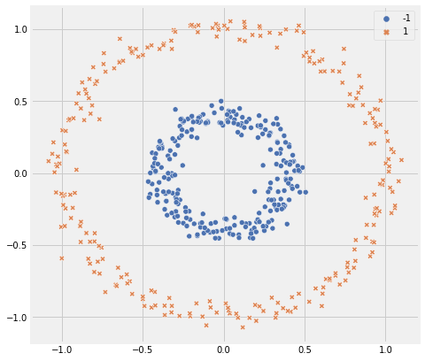
from sklearn.datasets import make_circles, make_swiss_roll

X, y = make_circles(n_samples=500, noise=0.05, shuffle=True, random_state=11, factor=0.4)
y = np.where(y == 0, 1, -1) # to change classes from 0, 1 to -1, 1

fig = plt.figure(figsize=(7,7))
ax = fig.add_subplot(1,1,1)
sns.scatterplot(x=X[:,0], y=X[:,1], hue=y, style=y, ax=ax, palette='deep')
plt.show()
Kernels#
Kernel Name |
Equation |
|---|---|
Linear |
\begin{align} K(x, z) &= x^T z \end{align} |
Radial Basis Function (RBF) / Gaussian Kernel |
\begin{align} K(x, z) &= e^{\big( - \frac{|| x - z ||^2}{2 \sigma^2}\big)} \text{ or } \gamma = \frac{1}{2 \sigma^2} \\ \\ K(x, z) &= e^{\big( - {\gamma || x - z ||^2}\big)} \end{align} |
Laplace |
\begin{align} K(x, z) &= e^{\big( - {\gamma | x - z |}\big)} \end{align} |
Sigmoid |
\begin{align} K(x, z) &= \tanh{(a x^T z + c)} \end{align} |
Polynomial |
\begin{align} K(x, z) &= (1 + x^T z)^d \end{align} |
Implementation#
[3]:
# np.random.seed(0)

class Kernel:
    def __init__(self, name):
        self.name = name

    def _rbf(self, X, gamma=2):
        return np.exp(-gamma * np.linalg.norm(X, axis=1, ord=2))

    def _laplace(self, X, gamma=2):
        return np.exp(-gamma * np.linalg.norm(X, axis=1, ord=1))

    def _linear(self, X):
        return X[:, 0] * X[:, 1]

    def _poly(self, X, d=3):
        return (1 + (X[:, 0] * X[:, 1]))**d

    def _sigmoid(self, X, a=3, c=1):
        return np.tanh((a * X[:, 0] * X[:, 1]) + c)

    def _parabolic(self, X):
        return X[:, 1]**2 - X[:, 0]**2

    def __call__(self, X, *args, **kwargs):
        if self.name == "rbf":
            return self._rbf(X, *args, **kwargs)
        if self.name == "laplace":
            return self._laplace(X, *args, **kwargs)
        elif self.name == "linear":
            return self._linear(X)
        elif self.name == "polynomial":
            return self._poly(X, *args, **kwargs)
        elif self.name == "sigmoid":
            return self._sigmoid(X, *args, **kwargs)
        else:
            print(f"Kernel {self.name} is not identified")
            return X
[4]:
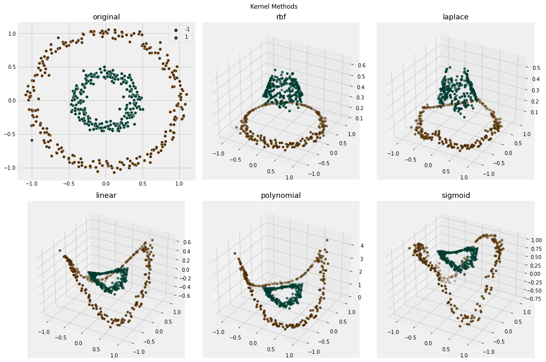
fig = plt.figure(figsize=(15, 10))


ax1 = fig.add_subplot(2, 3, 1)
sns.scatterplot(x=X[:, 0], y=X[:, 1], hue=y, ax=ax1, palette='BrBG_r')
ax1.set_title("original")

ax2 = fig.add_subplot(2, 3, 2, projection='3d')
trans_X = np.c_[X, Kernel('rbf')(X)]
ax2.scatter(trans_X[:, 0], trans_X[:, 1], trans_X[:, 2], c=y, cmap='BrBG_r')
ax2.set_title("rbf")

ax3 = fig.add_subplot(2, 3, 3, projection='3d')
trans_X = np.c_[X, Kernel('laplace')(X)]
ax3.scatter(trans_X[:, 0], trans_X[:, 1], trans_X[:, 2], c=y, cmap='BrBG_r')
ax3.set_title("laplace")

ax4 = fig.add_subplot(2, 3, 4, projection='3d')
trans_X = np.c_[X, Kernel('linear')(X)]
ax4.scatter(trans_X[:, 0], trans_X[:, 1], trans_X[:, 2], c=y, cmap='BrBG_r')
ax4.set_title("linear")

ax5 = fig.add_subplot(2, 3, 5, projection='3d')
trans_X = np.c_[X, Kernel('polynomial')(X)]
ax5.scatter(trans_X[:, 0], trans_X[:, 1], trans_X[:, 2], c=y, cmap='BrBG_r')
ax5.set_title("polynomial")

ax6 = fig.add_subplot(2, 3, 6, projection='3d')
trans_X = np.c_[X, Kernel('sigmoid')(X)]
ax6.scatter(trans_X[:, 0], trans_X[:, 1], trans_X[:, 2], c=y, cmap='BrBG_r')
ax6.set_title("sigmoid")

plt.suptitle("Kernel Methods")
plt.tight_layout()
plt.show()
[5]:
np.random.seed(0)

class SVM:
    def __init__(self, n_iter = 100, lambda_param = 0.01, learning_rate = 0.001,
                 kernel=None, kernel_args=None, kernel_kwargs=None):
        self.n_iter = n_iter
        self.lambda_param = lambda_param
        self.learning_rate = learning_rate
        self.w = None
        self.b = None
        self.l_loss = None
        self.kernel = kernel
        self.kernel_args = kernel_args or []
        self.kernel_kwargs = kernel_kwargs or {}

    @property
    def margin(self):
        # return 1 / np.linalg.norm(self.w, ord=2)
        return 1 / np.sqrt(np.sum(np.square(model.w)))

    @property
    def loss(self):
        return self.l_loss

    def _predict(self, X, *args, **kwargs):
        return np.sign((self.w @ X.T) + self.b)

    def predict(self, X):
        X = self._apply_kernel(X)
        return self._predict(X)

    def _apply_kernel(self, X):
        if self.kernel is not None:
            X = np.c_[X, Kernel(self.kernel)(X, *self.kernel_args, **self.kernel_kwargs)]
        return X


    def fit(self, X, y):
        X = self._apply_kernel(X)

        n_samples, n_features = X.shape

        self.w = np.zeros(n_features) #np.random.rand(n_features)
        self.b = 0
        self.l_loss = []
        self.l_margin = []

        for _ in range(self.n_iter):
            for i in range(n_samples):
                if (y[i] * ((self.w @ X[i].T) + self.b)) >= 1:
                    self.w = self.w - ( self.learning_rate * (2 * self.lambda_param * self.w))
                else:
                    self.w = self.w - ( self.learning_rate * (( 2 * self.lambda_param * self.w ) - (y[i] * X[i])))
                    self.b = self.b + ( self.learning_rate * y[i] )

                self.l_loss.append(metrics.hinge_loss(y, self._predict(X)))
                self.l_margin.append(self.margin)


    def plot_boundary_3d(self, X, ax=None):
        # np.random.seed(10)

        trans_X = self._apply_kernel(X)
        y_pred = self._predict(trans_X)
        margin = self.margin

        if ax is None:
            fig = plt.figure(figsize=(7, 7))
            ax = fig.add_subplot(1, 1, 1, projection='3d')
            ax.set_title("Dicision Boundary - Hyperplane")

        grid_samples = 100

        xx, yy = np.meshgrid(
            np.linspace(X[:, 0].min() - 1 , X[:, 0].max() + 1 , grid_samples),
            np.linspace(X[:, 1].min() - 1 , X[:, 1].max() + 1 , grid_samples)
        )
        mesh = np.c_[xx.ravel(), yy.ravel()]
        trans_mesh = self._apply_kernel(mesh)
        mesh_pred = (self.w @ trans_mesh.T) + self.b
        zz = mesh_pred.reshape(xx.shape)

        ax.plot_surface(xx, yy, zz, cmap='BrBG_r', alpha=0.2)
        ax.scatter(trans_X[:, 0], trans_X[:, 1], trans_X[:, 2], c=y, cmap='BrBG_r')

        # ax.legend()

    def plot_boundary(self, X, ax=None):
        # np.random.seed(10)

        y_pred = self.predict(X)
        margin = self.margin

        if ax is None:
            fig, ax = plt.subplots(1, 1, figsize=(7, 7))
            ax.set_title("Dicision Boundary - Hyperplane")

        grid_samples = 100

        xx, yy = np.meshgrid(
            np.linspace(X[:, 0].min() - 1 , X[:, 0].max() + 1 , grid_samples),
            np.linspace(X[:, 1].min() - 1 , X[:, 1].max() + 1 , grid_samples)
        )
        mesh = np.c_[xx.ravel(), yy.ravel()]
        mesh_pred = self.predict(mesh)
        zz = mesh_pred.reshape(xx.shape)

        ax.contourf(xx, yy, zz, cmap=plt.cm.coolwarm, alpha=0.2)
        sns.scatterplot(x=X[:, 0], y=X[:, 1], hue=y, style=y, ax=ax, palette='deep')

        ax.legend()

    def plot_loss(self, ax=None):
        if ax is None:
            fig, ax = plt.subplots(1, 1, figsize=(7, 7))
            ax.set_title("Loss over iterations")

        ax.plot(self.loss)


    def plot_margin(self, ax=None):
        if ax is None:
            fig, ax = plt.subplots(1, 1, figsize=(7, 7))
            ax.set_title("Margin over iterations")

        ax.plot(self.l_margin)


    def plot(self, X):
        fig = plt.figure(figsize=(15, 5))

        ax1 = fig.add_subplot(1, 3, 1)
        self.plot_boundary(X, ax=ax1)
        ax1.set_title("Dicision Boundary - Hyperplane")

        ax2 = fig.add_subplot(1, 3, 2)
        self.plot_loss(ax=ax2)
        ax2.set_title("Loss over iterations")

        ax3 = fig.add_subplot(1, 3, 3)
        self.plot_margin(ax=ax3)
        ax3.set_title("Margin over iterations")
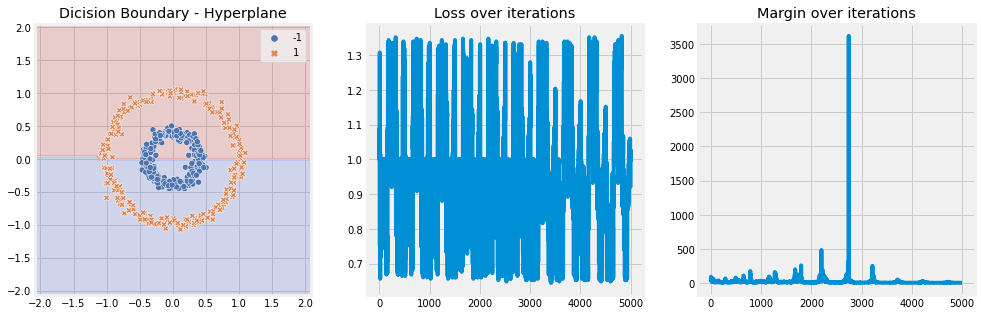
Without Kernel#
[6]:
model = SVM(n_iter=10, lambda_param=0.001, learning_rate=0.01)
model.fit(X, y)
model.plot(X)
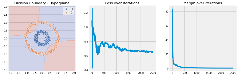
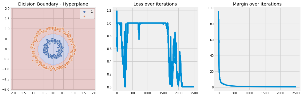
RBF Kernel#
[13]:
model = SVM(n_iter=5, lambda_param=0.001, learning_rate=0.01, kernel='rbf', kernel_kwargs={"gamma" : 2})
model.fit(X, y)

model.plot(X)
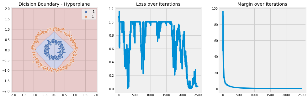
Laplace Kernel#
[8]:
model = SVM(n_iter=5, lambda_param=0.001, learning_rate=0.01, kernel='laplace')
model.fit(X, y)

model.plot(X)
Polynomial Kernel#
[9]:
model = SVM(n_iter=5, lambda_param=0.001, learning_rate=0.01, kernel='polynomial', kernel_kwargs={"d" : 2})
model.fit(X, y)

model.plot(X)
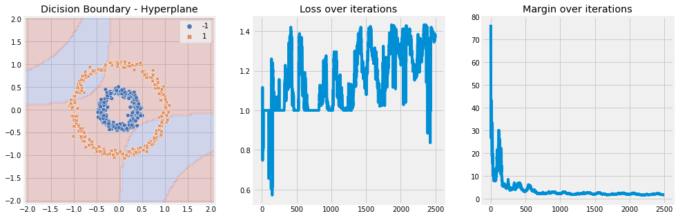
Linear Kernel#
[10]:
model = SVM(n_iter=5, lambda_param=0.001, learning_rate=0.01, kernel='linear')
model.fit(X, y)

model.plot(X)
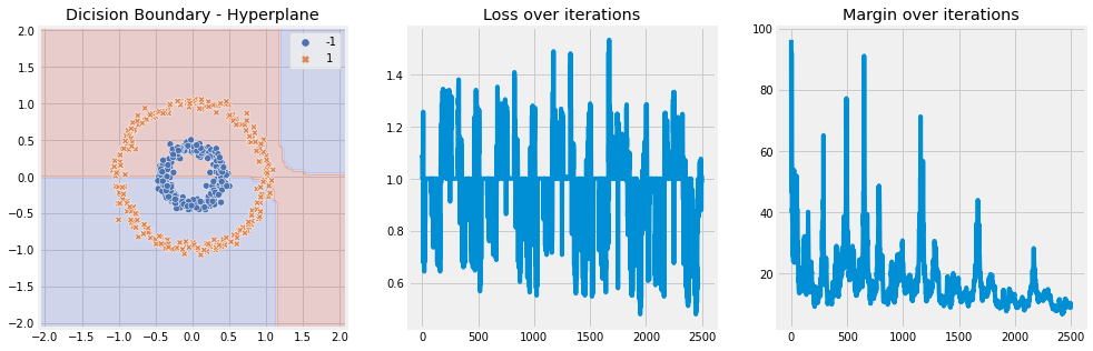
Sigmoid Kernel#
[11]:
model = SVM(n_iter=5, lambda_param=0.001, learning_rate=0.01, kernel='sigmoid')
model.fit(X, y)

model.plot(X)