Ridge(L2 Regularization) Regression#
References#
https://www.youtube.com/watch?v=Q81RR3yKn30 (statquest)
https://www.youtube.com/watch?v=QjOILAQ0EFg (Andrew NG)
Theory#
When sample sizes are relatively small then Ridge Regression can improve predictions made from new data (introducing bias and reducing variance) by making predictions less sensitive to training data.
Even when there is no enough data to find least square solution, ridge regression can find a solution using cross validation and penalty.
Generate Data#
[1]:
import pandas as pd
import numpy as np
from sklearn.datasets import make_regression
import matplotlib.pyplot as plt
from mpl_toolkits import mplot3d
import seaborn as sns

from matplotlib import animation
from IPython import display

from utility import regression_plot, regression_animation
[2]:
def add_axis_for_bias(X_i):
    m, n = X_i.shape
    if False in (X_i[:,0] == 1):
        return np.c_[np.ones(m) , X_i]
    else:
        return X_i
[3]:
sample_size = 100
train_size = 0.7 #70%
X, y = make_regression(n_samples=sample_size, n_features=1, noise=20, random_state=0)
y = y.reshape(-1, 1)
np.random.seed(10)
random_idxs = np.random.permutation(np.arange(0, sample_size))[: int(np.ceil(sample_size * train_size))]
X_train, y_train = X[random_idxs], y[random_idxs]
X_test, y_test = np.delete(X, random_idxs).reshape(-1, 1), np.delete(y, random_idxs).reshape(-1, 1)
### introduce bias in test data
bias = -50
X_r, y_r = make_regression(n_samples=20, n_features=1, noise=5, bias=bias, random_state=0)
X_test, y_test = np.r_[X_test, X_r], np.r_[y_test, y_r.reshape(-1, 1)]
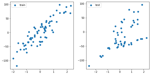
fig, ax = plt.subplots(1, 2, figsize=(10, 5))
ax[0].plot(X_train, y_train, 'o', label='train')
ax[0].legend()
ax[1].plot(X_test, y_test, 'o', label='test')
ax[1].legend()
plt.show()

Ridge with Normal Equation#
Loss Function#
\begin{align} L(\theta) = ||y - X\theta||^2 + \lambda ||\theta||^2 \end{align}
[4]:
def calculate_cost(X, y, theta, penalty):
    return np.linalg.norm(y - predict(X, theta)) + (penalty * np.square(np.linalg.norm(theta)))
Algorithm#
\begin{align} \text{If } X &= \text{independent variables}\\ y &= \text{dependent variable}\\ \lambda &= \text{penalty} \\ \text{then } \theta &= \text{predictor} = (X^T X + \lambda I)^{-1} X^T y\\ \\ \end{align}
[5]:
def ridge_regression_normaleq(X, y, penalty=1.0):
    X = add_axis_for_bias(X)
    m, n = X.shape
    theta = np.linalg.inv(X.T @ X + (penalty * np.eye(n))) @ X.T @ y
    return theta
[6]:
def predict(X, theta):
    format_X = add_axis_for_bias(X)
    if format_X.shape[1] == theta.shape[0]:
        y_pred = format_X @ theta # (m,1) = (m,n) * (n,1)
        return y_pred
    elif format_X.shape[1] == theta.shape[1]:
        y_pred = format_X @ theta.T # (m,1) = (m,n) * (n,1)
        return y_pred
    else:
        raise ValueError("Shape is not proper.")
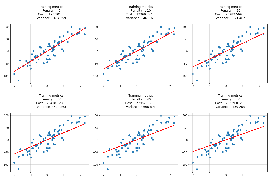
Training#
[7]:
penalty_list = np.arange(0, 51, 10)
penalty_list
[7]:
array([ 0, 10, 20, 30, 40, 50])
[8]:
cost_list = []
variance_list = []

cols = 3
rows = np.int32(np.ceil(len(penalty_list)/ cols))

fig, ax = plt.subplots(rows, cols, figsize=(cols*5, rows*5))
ax = ax.ravel()


for idx, penalty in enumerate(penalty_list):
    theta = ridge_regression_normaleq(X_train, y_train, penalty=penalty)
    y_hat = predict(X_train, theta)
    cost = calculate_cost(X_train, y_train, theta, penalty)
    variance = (y_train - y_hat).var(ddof=1)

    cost_list.append(cost)
    variance_list.append(variance)

    ax[idx].scatter(X_train, y_train)
    ax[idx].plot(X_train, y_hat, c='r')

    ax[idx].set_title(f"""
    Training metrics
    Penalty   : {penalty}
    Cost  : {round(cost, 3)}
    Variance  : {round(variance, 3)}
    """)
    ax[idx].grid(alpha=0.5)

plt.tight_layout()
plt.show()
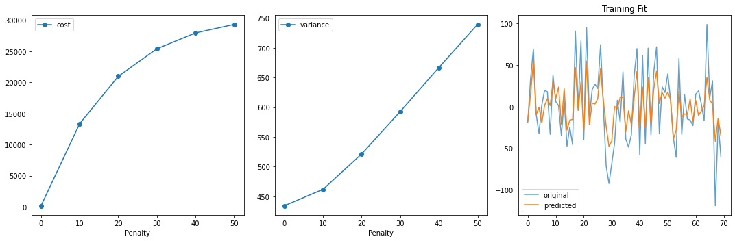
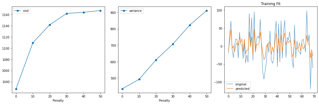
[9]:
fig, ax = plt.subplots(1, 3, figsize=(15, 5))
ax[0].plot(penalty_list, cost_list, 'o-', label='cost')
ax[0].set_xlabel("Penalty")
ax[0].legend()

ax[1].plot(penalty_list, variance_list, 'o-', label='variance')
ax[1].set_xlabel("Penalty")
ax[1].legend()

ax[2].plot(y_train, '-', label='original', alpha=0.7)
ax[2].plot(y_hat, '-', label='predicted')
ax[2].legend()
ax[2].set_title("Training Fit")

plt.tight_layout()
plt.show()
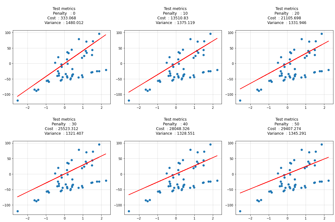
Evaluation On Test Data#
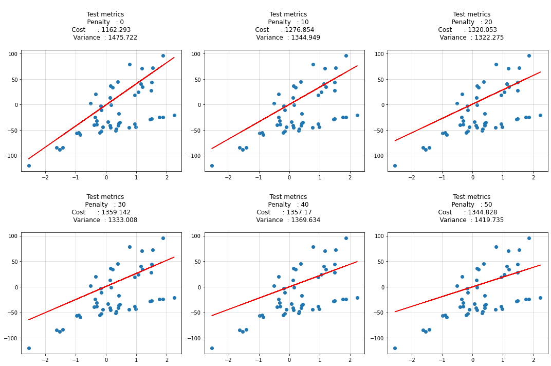
[10]:
cost_list = []
pred_list = []
variance_list = []
cols = 3
rows = np.int32(np.ceil(len(penalty_list)/ cols))
fig, ax = plt.subplots(rows, cols, figsize=(cols*5, rows*5))
ax = ax.ravel()
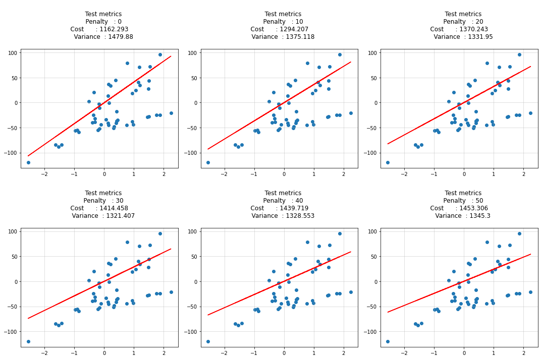
for idx, penalty in enumerate(penalty_list):
theta = ridge_regression_normaleq(X_train, y_train, penalty=penalty)
y_hat = predict(X_test, theta)
cost = calculate_cost(X_test, y_test, theta, penalty)
variance = (y_test - y_hat).var(ddof=1)
pred_list.append(y_hat[:, 0])
cost_list.append(cost)
variance_list.append(variance)
ax[idx].scatter(X_test, y_test)
ax[idx].plot(X_test, y_hat, c='r')
ax[idx].set_title(f"""
Test metrics
Penalty : {penalty}
Cost : {round(cost, 3)}
Variance : {round(variance, 3)}
""")
ax[idx].grid(alpha=0.5)
plt.tight_layout()
plt.show()
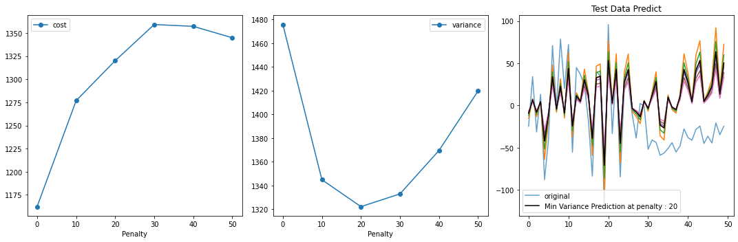
[11]:
fig, ax = plt.subplots(1, 3, figsize=(15, 5))
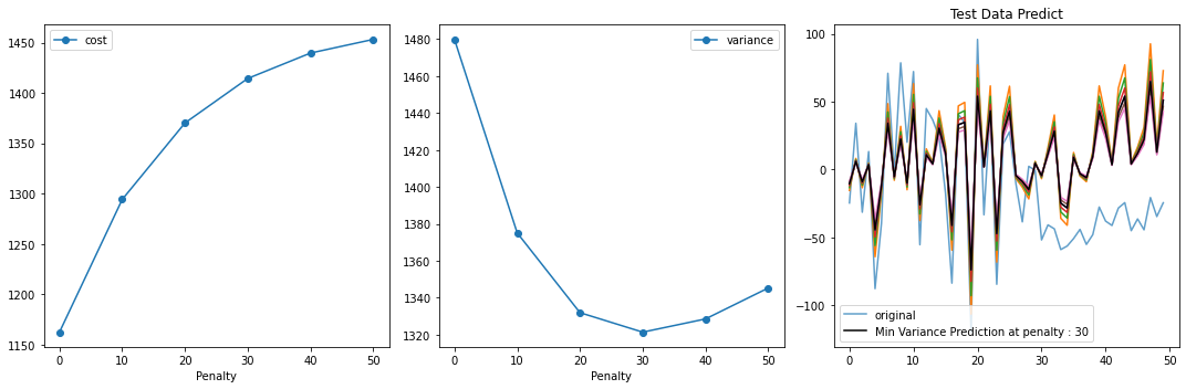
ax[0].plot(penalty_list, cost_list, 'o-', label='cost')
ax[0].set_xlabel("Penalty")
ax[0].legend()
ax[1].plot(penalty_list, variance_list, 'o-', label='variance')
ax[1].set_xlabel("Penalty")
ax[1].legend()
ax[2].plot(y_test, '-', label='original', alpha=0.7)
for i in pred_list:
ax[2].plot(i, '-')
min_var_idx = np.array(variance_list).argmin()
ax[2].plot(pred_list[min_var_idx], 'k-', label=f'Min Variance Prediction at penalty : {penalty_list[min_var_idx]}')
ax[2].legend()
ax[2].set_title("Test Data Predict")
plt.tight_layout()
plt.show()
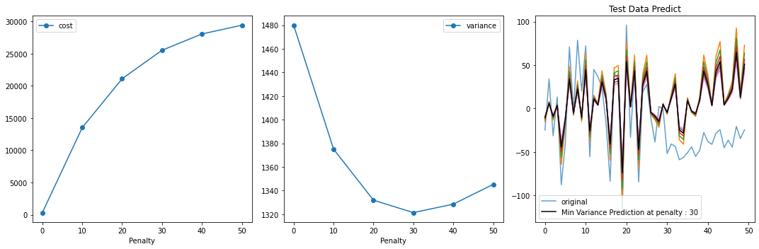
As I have introduced a bias in test data. that is not present in training data. but still based on my prior knowledge I introduced a penality in the learning algorithm. with increasing penalty variance in testing decreased and bias increased.
It might not be the best fit for training. but it stops from overfitting and out of time validation/real data/test data evaulation is improved.
Ridge with BGD#
Going to use the same data
[12]:
fig, ax = plt.subplots(1, 2, figsize=(10, 5))
ax[0].plot(X_train, y_train, 'o', label='train')
ax[0].legend()
ax[1].plot(X_test, y_test, 'o', label='test')
ax[1].legend()
plt.show()
Cost Function#
\begin{align} J(\theta) &= \frac{1}{2m} \big[{\sum_{i=1}^{m}(h_{\theta}(x^{(i)}) - y^{(i)})^2 + \lambda \sum_{j=1}^{n}{\theta_j^2}} \big] \\ \end{align}
[13]:
def calculate_cost(y_pred, y, penalty, theta):
    m = y.shape[0]
    return (np.square(y_pred - y).sum()/(2 * m)) + (penalty * np.square(theta).sum()/(2 * m))
Derivative#
\begin{align} \text{derivative} = \frac{\partial{J(\theta)}}{\partial{\theta}} &= \frac{1}{m}{\sum_{i=1}^{m}{(h_\theta(x^{(i)}) - y^{(i)})}}.{x_j^{(i)}} + \frac{\lambda}{m}{\theta_j} \end{align}
[14]:
def derivative(X, y, y_pred, penalty, theta):
    m, _ = X.shape
    base_grad = np.sum( ( y_pred - y ) * X, axis = 0 ) / m
    penalty_grad = (penalty * theta).sum(axis=0) / m
    penalty_grad[0] = 0 #for theta 0 penalty is 0
    return base_grad + penalty_grad
Algorithm#
\begin{align} \text{repeat until convergence \{}\\ \theta_0 &:= \theta_0 - \alpha \frac{1}{m}{\sum_{i=1}^{m}{(h_\theta(x^{(i)}) - y^{(i)})}}.x_0^{(i)}\\ \theta_j &:= \theta_j - \alpha \big{[} \frac{1}{m}{\sum_{i=1}^{m}{(h_\theta(x^{(i)}) - y^{(i)})}}.{x_j^{(i)}} + \frac{\lambda}{m}{\theta_j} \big{]}\\ \text{\} j = 1,2,3,...,n} \end{align}
[15]:
def predict(X, theta):
    format_X = add_axis_for_bias(X)

    if format_X.shape[1] == theta.shape[0]:
        y_pred = format_X @ theta # (m,1) = (m,n) * (n,1)
        return y_pred
    elif format_X.shape[1] == theta.shape[1]:
        y_pred = format_X @ theta.T # (m,1) = (m,n) * (n,1)
        return y_pred
    else:
        raise ValueError("Shape is not proper.")
[16]:
def ridge_regression_bgd(X, y, verbose=True, theta_precision = 0.001, alpha = 0.01,
                         iterations = 10000, penalty=1.0):

    X = add_axis_for_bias(X)
    m, n = X.shape

    theta_history = []
    cost_history = []

    # number of features+1 because of theta_0
    theta = np.random.rand(1,n) * theta_precision

    for iteration in range(iterations):

        theta_history.append(theta[0])

        # calculate y_pred
        y_pred = X @ theta.T

        # simultaneous operation
        gradient = derivative(X, y, y_pred, penalty, theta)
        theta = theta - (alpha * gradient)


        if np.isnan(np.sum(theta)) or np.isinf(np.sum(theta)):
            print(f"breaking at iteration {iteration}. found inf or nan.")
            break

        # calculate cost to put in history
        cost = calculate_cost(predict(X, theta), y, penalty, theta)
        cost_history.append(cost)

    return theta, np.array(theta_history), np.array(cost_history)
Training#
[17]:
penalty_list = np.arange(0, 51, 10)
penalty_list
[17]:
array([ 0, 10, 20, 30, 40, 50])
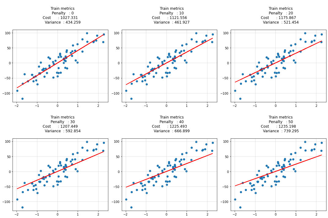
[18]:
cost_list = []
bias_list = []
variance_list = []
cols = 3
rows = np.int32(np.ceil(len(penalty_list)/ cols))
fig, ax = plt.subplots(rows, cols, figsize=(cols*5, rows*5))
ax = ax.ravel()
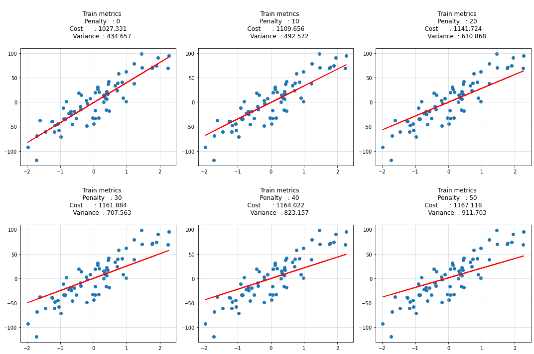
for idx, penalty in enumerate(penalty_list):
theta, _, _ = theta, theta_history, cost_history = ridge_regression_bgd(
X_train, y_train, verbose=True, theta_precision = 0.001,
alpha = 0.03, iterations = 300,
penalty = penalty
)
y_hat = predict(X_train, theta)
cost = calculate_cost(X_train, y_train, penalty, theta)
variance = (y_train - y_hat).var(ddof=1)
bias_list.append(theta[0][0])
cost_list.append(cost)
variance_list.append(variance)
ax[idx].scatter(X_train, y_train)
ax[idx].plot(X_train, y_hat, c='r')
ax[idx].set_title(f"""
Train metrics
Penalty : {penalty}
Cost : {round(cost, 3)}
Variance : {round(variance, 3)}
""")
ax[idx].grid(alpha=0.5)
plt.tight_layout()
plt.show()
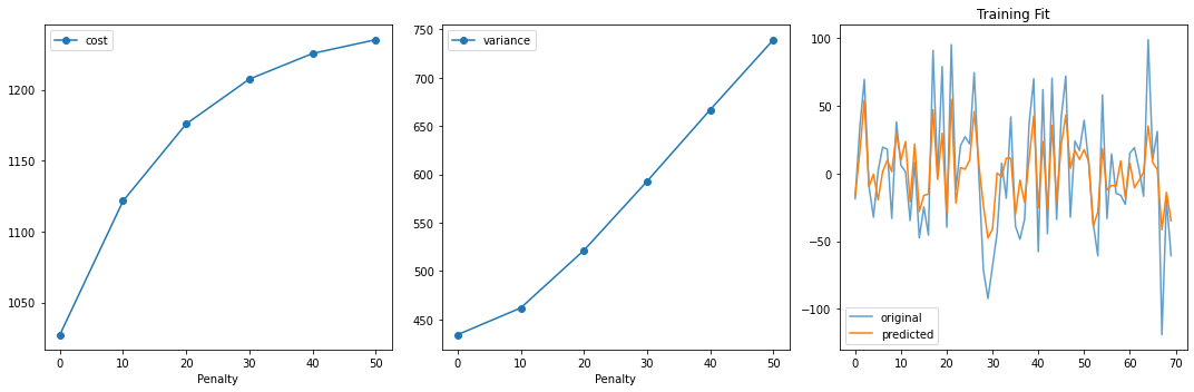
[19]:
fig, ax = plt.subplots(1, 3, figsize=(15, 5))
ax[0].plot(penalty_list, cost_list, 'o-', label='cost')
ax[0].set_xlabel("Penalty")
ax[0].legend()

ax[1].plot(penalty_list, variance_list, 'o-', label='variance')
ax[1].set_xlabel("Penalty")
ax[1].legend()

ax[2].plot(y_train, '-', label='original', alpha=0.7)
ax[2].plot(y_hat, '-', label='predicted')
ax[2].legend()
ax[2].set_title("Training Fit")

plt.tight_layout()
plt.show()
Testing#
[20]:
penalty_list = np.arange(0, 51, 10)
penalty_list
[20]:
array([ 0, 10, 20, 30, 40, 50])
[21]:
cost_list = []
pred_list = []
variance_list = []

cols = 3
rows = np.int32(np.ceil(len(penalty_list)/ cols))

fig, ax = plt.subplots(rows, cols, figsize=(cols*5, rows*5))
ax = ax.ravel()


for idx, penalty in enumerate(penalty_list):
    theta, _, _ = theta, theta_history, cost_history = ridge_regression_bgd(
        X_train, y_train, verbose=True, theta_precision = 0.001,
        alpha = 0.03, iterations = 300,
        penalty = penalty
    )
    y_hat = predict(X_test, theta)
    cost = calculate_cost(X_test, y_test, penalty, theta)
    variance = (y_test - y_hat).var(ddof=1)

    pred_list.append(y_hat[:, 0])
    cost_list.append(cost)
    variance_list.append(variance)

    ax[idx].scatter(X_test, y_test)
    ax[idx].plot(X_test, y_hat, c='r')

    ax[idx].set_title(f"""
    Test metrics
    Penalty   : {penalty}
    Cost      : {round(cost, 3)}
    Variance  : {round(variance, 3)}
    """)
    ax[idx].grid(alpha=0.5)

plt.tight_layout()
plt.show()
[22]:
fig, ax = plt.subplots(1, 3, figsize=(15, 5))
ax[0].plot(penalty_list, cost_list, 'o-', label='cost')
ax[0].set_xlabel("Penalty")
ax[0].legend()

ax[1].plot(penalty_list, variance_list, 'o-', label='variance')
ax[1].set_xlabel("Penalty")
ax[1].legend()

ax[2].plot(y_test, '-', label='original', alpha=0.7)
for i in pred_list:
    ax[2].plot(i, '-')

min_var_idx = np.array(variance_list).argmin()
ax[2].plot(pred_list[min_var_idx], 'k-', label=f'Min Variance Prediction at penalty : {penalty_list[min_var_idx]}')
ax[2].legend()
ax[2].set_title("Test Data Predict")

plt.tight_layout()
plt.show()
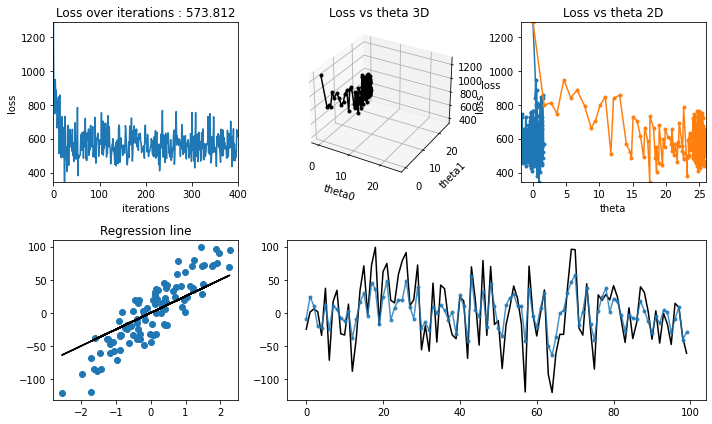
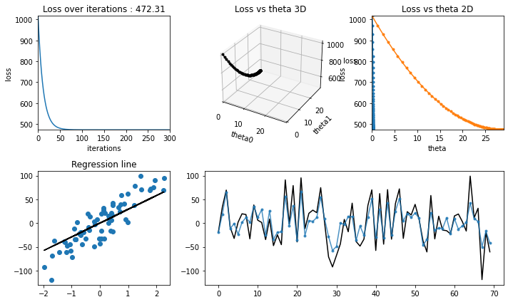
Training Animation#
[23]:
iterations = 300
learning_rate = 0.03
penalty = 30.0

theta, theta_history, cost_history = ridge_regression_bgd(
    X_train, y_train, verbose=True, theta_precision = 0.1,
    alpha = learning_rate, iterations = iterations,
    penalty = penalty
)

regression_animation(X_train, y_train, cost_history, theta_history, iterations, interval=10)
# regression_plot(X_train, y_train, cost_history, theta_history, iterations);
[23]:
Ridge with SGD#
Stochastic gradient descent (often abbreviated SGD) is an iterative method for optimizing an objective function with suitable smoothness properties (e.g. differentiable or subdifferentiable).
It can be regarded as a stochastic approximation of gradient descent optimization, since it replaces the actual gradient (calculated from the entire data set) by an estimate thereof (calculated from a randomly selected subset of the data).
Especially in high-dimensional optimization problems this reduces the computational burden, achieving faster iterations in trade for a lower convergence rate.
It is - an iterative method - train over random samples of a batch size instead of training on whole dataset - faster convergence on large dataset
Algorithm#
[24]:
def ridge_regression_sgd(X, y, verbose=True, theta_precision = 0.001, batch_size=30,
                         alpha = 0.01, iterations = 10000, penalty=1.0):

    X = add_axis_for_bias(X)
    m, n = X.shape

    theta_history = []
    cost_history = []

    # number of features+1 because of theta_0
    theta = np.random.rand(1,n) * theta_precision

    for iteration in range(iterations):

        theta_history.append(theta[0])

        indices = np.random.randint(0, m, size=batch_size)

        # creating batch for this iteration
        X_batch = X[indices,:]
        y_batch = y[indices,:]

        # calculate y_pred
        y_pred = X_batch @ theta.T

        # simultaneous operation
        gradient = derivative(X_batch, y_batch, y_pred, penalty, theta)
        theta = theta - (alpha * gradient)


        if np.isnan(np.sum(theta)) or np.isinf(np.sum(theta)):
            print(f"breaking at iteration {iteration}. found inf or nan.")
            break

        # calculate cost to put in history
        cost = calculate_cost(predict(X_batch, theta), y_batch, penalty, theta)
        cost_history.append(cost)

    return theta, np.array(theta_history), np.array(cost_history)
Training#
[25]:
penalty_list = np.arange(0, 51, 10)
penalty_list
[25]:
array([ 0, 10, 20, 30, 40, 50])
[26]:
cost_list = []
bias_list = []
variance_list = []

cols = 3
rows = np.int32(np.ceil(len(penalty_list)/ cols))

iterations = 400
learning_rate = 0.03
batch_size = 45

fig, ax = plt.subplots(rows, cols, figsize=(cols*5, rows*5))
ax = ax.ravel()


for idx, penalty in enumerate(penalty_list):
    theta, _, _ = theta, theta_history, cost_history = ridge_regression_sgd(
        X_train, y_train, verbose=True, theta_precision = 0.001,
        alpha = learning_rate, iterations = iterations, batch_size=batch_size,
        penalty = penalty
    )
    y_hat = predict(X_train, theta)
    cost = calculate_cost(X_train, y_train, penalty, theta)
    variance = (y_train - y_hat).var(ddof=1)

    bias_list.append(theta[0][0])
    cost_list.append(cost)
    variance_list.append(variance)

    ax[idx].scatter(X_train, y_train)
    ax[idx].plot(X_train, y_hat, c='r')

    ax[idx].set_title(f"""
    Train metrics
    Penalty   : {penalty}
    Cost      : {round(cost, 3)}
    Variance  : {round(variance, 3)}
    """)
    ax[idx].grid(alpha=0.5)

plt.tight_layout()
plt.show()
[27]:
fig, ax = plt.subplots(1, 3, figsize=(15, 5))
ax[0].plot(penalty_list, cost_list, 'o-', label='cost')
ax[0].set_xlabel("Penalty")
ax[0].legend()

ax[1].plot(penalty_list, variance_list, 'o-', label='variance')
ax[1].set_xlabel("Penalty")
ax[1].legend()

ax[2].plot(y_train, '-', label='original', alpha=0.7)
ax[2].plot(y_hat, '-', label='predicted')
ax[2].legend()
ax[2].set_title("Training Fit")

plt.tight_layout()
plt.show()
Testing#
[28]:
cost_list = []
pred_list = []
variance_list = []

cols = 3
rows = np.int32(np.ceil(len(penalty_list)/ cols))

iterations = 400
learning_rate = 0.03
batch_size = 45

fig, ax = plt.subplots(rows, cols, figsize=(cols*5, rows*5))
ax = ax.ravel()


for idx, penalty in enumerate(penalty_list):
    theta, _, _ = theta, theta_history, cost_history = ridge_regression_sgd(
        X_train, y_train, verbose=True, theta_precision = 0.001,
        alpha = learning_rate, iterations = iterations, batch_size = batch_size,
        penalty = penalty
    )
    y_hat = predict(X_test, theta)
    cost = calculate_cost(X_test, y_test, penalty, theta)
    variance = (y_test - y_hat).var(ddof=1)

    pred_list.append(y_hat[:, 0])
    cost_list.append(cost)
    variance_list.append(variance)

    ax[idx].scatter(X_test, y_test)
    ax[idx].plot(X_test, y_hat, c='r')

    ax[idx].set_title(f"""
    Test metrics
    Penalty   : {penalty}
    Cost      : {round(cost, 3)}
    Variance  : {round(variance, 3)}
    """)
    ax[idx].grid(alpha=0.5)

plt.tight_layout()
plt.show()
[29]:
fig, ax = plt.subplots(1, 3, figsize=(15, 5))
ax[0].plot(penalty_list, cost_list, 'o-', label='cost')
ax[0].set_xlabel("Penalty")
ax[0].legend()

ax[1].plot(penalty_list, variance_list, 'o-', label='variance')
ax[1].set_xlabel("Penalty")
ax[1].legend()

ax[2].plot(y_test, '-', label='original', alpha=0.7)
for i in pred_list:
    ax[2].plot(i, '-')

min_var_idx = np.array(variance_list).argmin()
ax[2].plot(pred_list[min_var_idx], 'k-', label=f'Min Variance Prediction at penalty : {penalty_list[min_var_idx]}')
ax[2].legend()
ax[2].set_title("Test Data Predict")

plt.tight_layout()
plt.show()
Training Animation#
[30]:
iterations = 400
learning_rate = 0.03
penalty = 30
batch_size = 45

theta, theta_history, cost_history = ridge_regression_sgd(X_train, y_train, verbose=True, theta_precision = 0.001, batch_size=45,
                                                           alpha = learning_rate, iterations = iterations, penalty=penalty)

regression_animation(X, y, cost_history, theta_history, iterations, interval=10)
# regression_plot(X_train, y_train, cost_history, theta_history, iterations);
[30]: