Time Series Forecasting#
WORK IN PROGRESS
References#
[1]:
from datetime import datetime

import numpy as np
import pandas as pd
import matplotlib.pyplot as plt
import seaborn as sns

from scipy.stats import spearmanr, pearsonr
from mightypy.ml import moving_window_matrix # This is my package
from graphpkg.static import plot_boxed_timeseries

plt.style.use('seaborn')
plt.rcParams.update({
    "figure.figsize" : (12, 8)
})
Introduction to Time Series#
\begin{align} \{X_1, X_2, ..., X_T\} \end{align}
Time series forecasting occurs when you make scientific predictions based on historical time stamped data. It involves building models through historical analysis and using them to make observations and drive future strategic decision-making.
Time series is any sequence record over time eg.- hourly, daily, weekly etc.
Some applications of Time Series -
Interpretation : make sense of the data and capture changes/ dynamics.
Modeling and Forecasting : Understanding aspects of data and create models for predictions/ future forecast.
Filtering/ Smoothing : Process the data.
Basic Model#
Timeseries data has this basic composition.
\begin{align} X_t &= T_t + S_t + C_t + I_t \end{align}
This represents an additive model, yeah I can see addition signs.
\begin{align} X_t &= T_t \times S_t \times C_t \times I_t \end{align} > This represents a multiplicative model.
Where
\(X_t\) = Trend : General direction of data. long-term progression of series.
\(S_t\) = Seasonal : component fixed and known period, distinct repeated patterns for regular intervals like yearly, quarterly, monthly, weekly etc. like sell count of xmas trees at the time of xmas.
\(C_t\) = Cyclical :
Optionalcomponent that is repeatative but doesn’t happen at fixed intervals.\(I_t\) = Residuals : fluctuations in time series after removing trend, seasonal and cyclic variations.
Each observation in the series can be expressed as either a sum or a product of the components.
More on this matter is explained in Seasonal Decomposition section.
Load Data#
[2]:
df = pd.read_csv('/opt/datasetsRepo/stock.csv')
Preprocessing#
[3]:
df['Date'] = df['Date'].apply(pd.to_datetime)
df['Close'] = df['Close'].apply(lambda x: float(x.replace(',','')))
df['Volume'] = df['Volume'].apply(lambda x: float(x.replace(',','')))
df.index = df['Date']

df.head(3)
[3]:
| Date | Open | High | Low | Close | Volume | |
|---|---|---|---|---|---|---|
| Date | ||||||
| 2012-01-03 | 2012-01-03 | 325.25 | 332.83 | 324.97 | 663.59 | 7380500.0 |
| 2012-01-04 | 2012-01-04 | 331.27 | 333.87 | 329.08 | 666.45 | 5749400.0 |
| 2012-01-05 | 2012-01-05 | 329.83 | 330.75 | 326.89 | 657.21 | 6590300.0 |
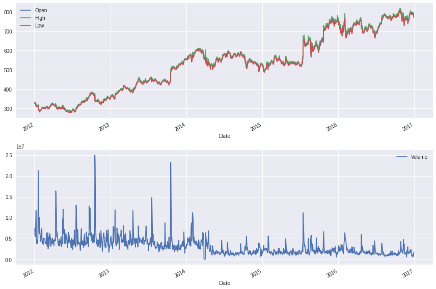
How does the data look like ?#
[4]:
fig, ax = plt.subplots(2,1)
df.plot(y=['Open','High','Low'], ax=ax[0])
df.plot(y=['Volume'], ax=ax[1])

plt.tight_layout()
plt.show()
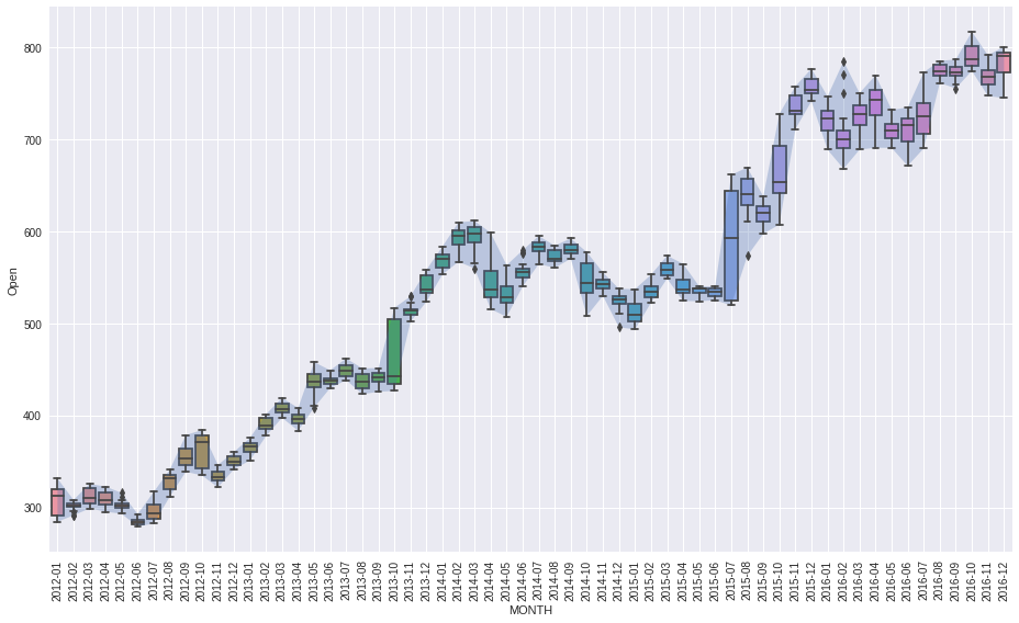
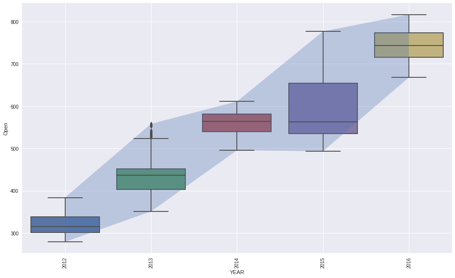
lets see monthly data stats using box plot#
[5]:
plot_boxed_timeseries(df=df, ts_col='Date', data_col='Open', box='month', figsize=(13,8))
plt.tight_layout()
plt.show()
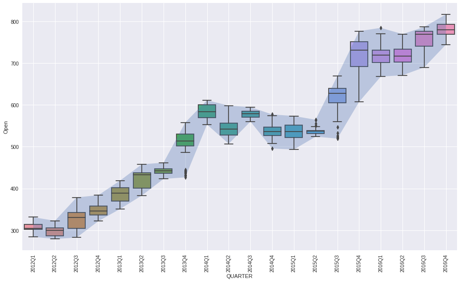
[6]:
plot_boxed_timeseries(df=df, ts_col='Date', data_col='Open', box='quarter', figsize=(13,8))
plt.tight_layout()
plt.show()
[16]:
plot_boxed_timeseries(df=df, ts_col='Date', data_col='Open', box='year', figsize=(13,8))
plt.tight_layout()
plt.show()
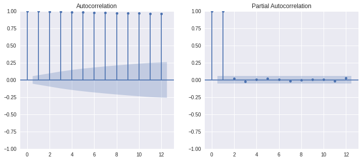
AutoCorrelation Function#
correlation between observations at the current timespot and the observations as previous timespots.
Partial AutoCorrelation Function#
[23]:
from statsmodels.graphics.tsaplots import plot_pacf, plot_acf
[29]:
LAGS = 12
data = df['Open']
fig, ax = plt.subplots(1,2, figsize=(12,5))
plot_acf(data, lags=LAGS, ax=ax[0])
plot_pacf(data, lags=LAGS, method='ywm', ax=ax[1]); plt.show()
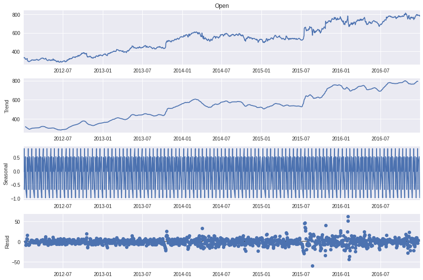
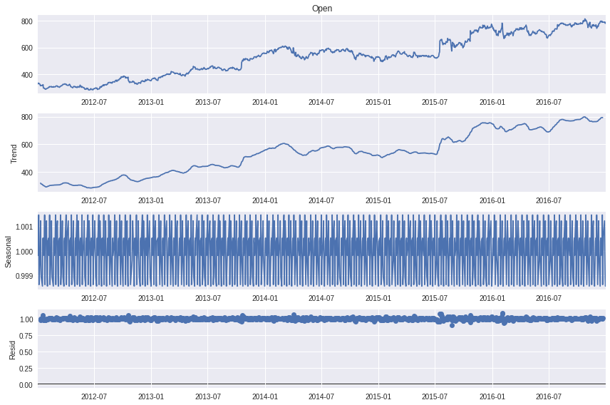
Seasonal Decompostion#
[12]:
from statsmodels.tsa.seasonal import seasonal_decompose
[13]:
data = df['Open']
Multiplicative Model#
\begin{align} X_t &= T_t \times S_t \times C_t \times I_t\\ \log{X_t} &= \log{T_t} + \log{S_t} + \log{C_t} + \log{I_t} \end{align}
[14]:
decomposition = seasonal_decompose(data, period=12, model='muplicative')
fig = decomposition.plot()
plt.show()
Additive Model#
[15]:
decomposition = seasonal_decompose(data, period=12, model='additive')
fig = decomposition.plot()
plt.show()