Logistic Regression#
Logistic regression is a statistical model that in its basic form uses a logistic function to model a binary dependent variable, although many more complex extensions exist. In regression analysis, logistic regression (or logit regression) is estimating the parameters of a logistic model (a form of binary regression).
given x, find \(\hat{y} = p(y=1 | x)\)
where \(0 \leq \hat{y} \leq 1\) and \(x \in R^{n_x}\)
Parameters : \(w \in R^{n_x}\), \(b \in R\)
Output : \(\hat{y} = \sigma(w^T x + b)\)
[1]:
import numpy as np
import pandas as pd
import matplotlib.pyplot as plt
from mpl_toolkits import mplot3d
import seaborn as sns
[2]:
def linear_model_format_X(X):
    if len(X.shape) == 1:
        X = X.copy().reshape(-1,1)

    return np.hstack(tup= ( np.ones(shape=(X.shape[0],1)) , X ) )
Cost Function#
The cross-entropy loss function#
We need a loss function that expresses, for an observationx, how close the classifier output
\(\hat{y} = σ(w^T x+b)\)
is to the correct output (y, which is 0 or 1). We’ll call this:
\(L(\hat{y},y)\) = How much \(\hat{y}\) differs from the true \(y\)
We do this via a loss function that prefers the correct class labels of the training examples to bemore likely. This is called conditional maximum likelihood estimation: we choose the parametersw,b thatmaximize the log probability ofthe true y labels in the training datagiven the observations x. The resulting loss function is the negative log likelihood loss, generally called the cross-entropy loss.
\(J(\theta)=\frac{1}{m} {\sum_{i=0}^{m}cost(h_{\theta}(x^{(i)}),y^{(i)})}\)
for non linear paramter there can be many local minima
\(cost(h_{\theta}(x), y) = \begin{cases} -\log(h_{\theta}(x)) & \text{if } y=1\\ -\log(1 - h_{\theta}(x)) & \text{if } y=0\\ \end{cases}\)
\(cost(h_{\theta}(x), y) = -y \log(h_{\theta}(x)) - (1 - y)\log(1 - h_{\theta}(x))\)
\(J(\theta) = -\frac{1}{m}{\sum_{i=0}^{m} \big[ y^{(i)} \log(h_{\theta}(x^{(i)})) - (1 - y^{(i)}) \log(1 - h_{\theta}(x^{(i)})) \big] }\)
MAXIMUM LIKELIHOOD ESTIMATION
[3]:
def calculate_entropy_cost(y_pred,y):
    m = y_pred.shape[0]
    part_1 = y * np.log(y_pred)

    part_2 = (1 - y) * np.log(1 - y_pred)

    cost = ( -1 / m ) * np.sum(part_1 + part_2)
    return cost
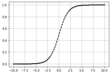
Sigmoid Function#
\(\sigma(z)= \frac{1}{1 + e^{-z}}\)
if z is positive large \(\sigma(z) \approx \frac{1}{1 + 0} \approx 1\)
if z is negative large \(\sigma(x) = \frac{1}{1 + e^{-z}} \approx 0\) here \(e^{-z}\) is a very big number
in case of hypothesis \(h_{\theta}(x) = \frac{1}{1 + e^{- \theta^T x}}\)
[4]:
def sigmoid(z):
    return 1 / (1 + np.exp(-z))
[5]:
data = np.linspace(-10,10,100)
plt.plot(data, sigmoid(data),'k.-',alpha=0.6)
plt.grid()
Gradient Descent Algorithm#
minimize \(J(\theta) \rightarrow\) get new theta \(\theta \rightarrow\) calculate \(h_{\theta}(x) = \frac{1}{1 + e^{-\theta^T x}} \rightarrow\) minimize \(J(\theta)\)
\begin{align} \text{repeat until convergence \{}\\ \theta_j &:= \theta_j - \alpha \frac{\partial}{\partial \theta_j} J(\theta)\\ \text{\}}\\ \end{align}
\(\frac {\partial}{\partial\theta_j} \bigg[-\frac{1}{m}{\sum_{i=0}^{m} \big[ y^{(i)} \log(h_{\theta}(x^{(i)})) - (1 - y^{(i)}) \log(1 - h_{\theta}(x^{(i)})) \big]} \bigg]\)
Math for Gradient Descent#
\begin{align} L &= -\frac{1}{m}{\sum_{i=1}^{m} \big[ y^{(i)} \log\hat{y} - (1 - y^{(i)}) \log(1 - \hat{y} ) \big]}\\ \hat{y} &= \frac{1}{1 + e^{- h_{\theta}(x)}}\\ h_{\theta}(x) &= \theta^T x\\ \\ \hat{y} & \text{ depends on } \theta\\ y & \text{ doesn't depend on } \theta \end{align}
task is to calculate
\(\frac{\partial L }{\partial \theta} = -\frac{1}{m} \frac{\partial}{\partial \theta} \big( y \log{\hat{y}} + (1 - y) \log{(1 - \hat{y})} \big)\)
\begin{align} \frac{\partial \hat{y}}{\partial \theta} &= \frac{\partial}{\partial \theta} \big( \frac{1}{1 + e^{-h_{\theta}(x)}} \big)\\ &= - \frac{1}{(1 + e^{-h_{\theta}(x)})^2} \frac{\partial}{\partial \theta} (1 + e^{-h_{\theta}(x)})\\ &= \frac{e^{-h_{\theta}(x)} x}{(1 + e^{-h_{\theta}(x)})^2}\\ &= \hat{y}^2 e^{-h_{\theta}(x)} x \\ \\ \frac{\partial L }{\partial \theta} =& -\frac{1}{m} \frac{\partial}{\partial \theta} \big( y \log{\hat{y}} + (1 - y) \log{(1 - \hat{y})} \big)\\ =& -\frac{1}{m} \bigg[ \frac{\partial}{\partial \theta} ( y \log{\hat{y}}) + \frac{\partial}{\partial \theta}((1 - y) \log{(1 - \hat{y})}) \bigg]\\ =& -\frac{1}{m} \bigg[ \frac{y}{\hat{y}} \frac{\partial}{\partial \theta} \hat{y} + \frac{(1 - y)}{(1 - \hat{y})} \frac{\partial}{\partial \theta}(1 - \hat{y}) \bigg]\\ =& -\frac{1}{m} \bigg[ \frac{y}{\hat{y}} \frac{\partial}{\partial \theta} \hat{y} - \frac{(1 - y)}{(1 - \hat{y})} \frac{\partial}{\partial \theta} \hat{y} \bigg]\\ =& -\frac{1}{m} \bigg[ \frac{y}{\hat{y}} \hat{y}^2 e^{-h_{\theta}(x)} x - \frac{(1 - y)}{(1 - \hat{y})} \hat{y}^2 e^{-h_{\theta}(x)} x \bigg]\\ \\ \\ 1 - \hat{y} &= 1 - \frac{1}{1 + e^{-h_{\theta}(x)}}\\ &= \frac{1 + e^{-h_{\theta}(x)} - 1}{1 + e^{-h_{\theta}(x)}}\\ &= \hat{y} e^{-h_{\theta}(x)}\\ \\ \\ \frac{\partial L }{\partial \theta} =& -\frac{1}{m} \bigg[ \frac{y}{\hat{y}} \hat{y}^2 e^{-h_{\theta}(x)} x - \frac{(1 - y)}{\hat{y} e^{-h_{\theta}(x)}} \hat{y}^2 e^{-h_{\theta}(x)} x \bigg]\\ =& -\frac{1}{m} \bigg[ \frac{y}{\hat{y}} \hat{y}^2 e^{-h_{\theta}(x)} x - \frac{(1 - y)}{\hat{y} e^{-h_{\theta}(x)}} \hat{y}^2 e^{-h_{\theta}(x)} x \bigg]\\ =& -\frac{1}{m} \bigg[ y \hat{y} e^{-h_{\theta}(x)} x - (1 - y)\hat{y} x \bigg]\\ =& -\frac{1}{m} \bigg[ y \hat{y} e^{-h_{\theta}(x)} x - \hat{y} x + y\hat{y} x \bigg]\\ =& -\frac{1}{m} \bigg[ y \hat{y} e^{-h_{\theta}(x)} - \hat{y} + y\hat{y} \bigg]x\\ =& -\frac{1}{m} \bigg[ y \hat{y}(1 + e^{-h_{\theta}(x)}) - \hat{y} \bigg]x\\ \frac{\partial L }{\partial \theta} =& -\frac{1}{m} \bigg[ y - \hat{y} \bigg]x \end{align}
[6]:
class LogisticRegression:
    def __init__(self,alpha = 0.01 ,iterations = 10000):
        self.alpha = alpha
        self.iterations = iterations
        self._theta = None
        self._X = None
        self._y = None
        self._theta_history = None
        self._cost_history = None

    def _format_X_for_theta_0(self,X_i):

        X_i = X_i.copy()
        if len(X_i.shape) == 1:
            X_i = X_i.reshape(-1,1)

        if False in (X_i[...,0] == 1):
            return np.hstack(tup=(np.ones(shape=(X_i.shape[0],1)) , X_i))
        else:
            return X_i

    @property
    def X(self):
        return self._X

    @property
    def y(self):
        return self._y

    @property
    def theta(self):
        return self._theta

    @property
    def theta_history(self):
        return self._theta_history

    @property
    def cost_history(self):
        return self._cost_history

    def predict(self,X):
        format_X = self._format_X_for_theta_0(X)

        if format_X.shape[1] == self._theta.shape[0]:
            y_pred = sigmoid(format_X @ self._theta) # (m,1) = (m,n) * (n,1)
            return y_pred
        elif format_X.shape[1] == self._theta.shape[1]:
            y_pred = sigmoid(format_X @ self._theta.T) # (m,1) = (m,n) * (n,1)
            return y_pred
        else:
            raise ValueError("Shape is not proper.")


    def train(self, X, y, verbose=True, method="BGD", theta_precision = 0.001, batch_size=30, regularization=False, penalty=1.0):

        self._X = self._format_X_for_theta_0(X)
        self._y = y

        # number of features+1 because of theta_0
        self._n = self._X.shape[1]
        self._m = self._y.shape[0]

        self._theta_history = []
        self._cost_history = []

        if method == "BGD":
            self._theta = np.random.rand(1,self._n) * theta_precision
            if verbose: print("random initial θ value :",self._theta)

            for iteration in range(self.iterations):
                # calculate y_pred
                y_pred = self.predict(self._X)

                # new θ to replace old θ
                new_theta = None

                # simultaneous operation

                if regularization:
                    gradient = np.mean( ( y_pred - self._y ) * self._X, axis = 0 )
                    new_theta_0 = self._theta[:,[0]] - (self.alpha *  gradient[0])
                    new_theta_rest = self._theta[:,range(1,self._n)] * (1 - (( self.alpha * penalty)/self._m) ) - (self.alpha *  gradient[1:])
                    new_theta = np.hstack((new_theta_0,new_theta_rest))

                else:
                    gradient = np.mean( ( y_pred - self._y ) * self._X, axis = 0 )
                    new_theta = self._theta - (self.alpha *  gradient)

                if np.isnan(np.sum(new_theta)) or np.isinf(np.sum(new_theta)):
                    print("breaking. found inf or nan.")
                    break
                # override with new θ
                self._theta = new_theta

                # calculate cost to put in history
                cost = calculate_entropy_cost(y_pred = self.predict(X=self._X), y = self._y)
                self._cost_history.append(cost)

                # calcualted theta in history
                self._theta_history.append(self._theta[0])

        elif method == "SGD": # stochastic gradient descent
            self._theta = np.random.rand(1,self._n) * theta_precision
            if verbose: print("random initial θ value :",self._theta)

            for iteration in range(self.iterations):

                # creating indices for batches
                indices = np.random.randint(0,self._m,size=batch_size)

                # creating batch for this iteration
                X_batch = np.take(self._X,indices,axis=0)
                y_batch = np.take(self._y,indices,axis=0)

                # calculate y_pred
                y_pred = self.predict(X_batch)
                # new θ to replace old θ
                new_theta = None

                # simultaneous operation
                if regularization:
                    gradient = np.mean( ( y_pred - y_batch ) * X_batch, axis = 0 )
                    new_theta_0 = self._theta[:,[0]] - (self.alpha *  gradient[0])
                    new_theta_rest = self._theta[:,range(1,self._n)] * (1 - (( self.alpha * penalty)/self._m) ) - (self.alpha *  gradient[1:])
                    new_theta = np.hstack((new_theta_0,new_theta_rest))


                else:
                    gradient = np.mean( ( y_pred - y_batch ) * X_batch, axis = 0 )
                    new_theta = self._theta - (self.alpha *  gradient)

                if np.isnan(np.sum(new_theta)) or np.isinf(np.sum(new_theta)):
                    print("breaking. found inf or nan.")
                    break
                # override with new θ
                self._theta = new_theta

                # calculate cost to put in history
                cost = calculate_entropy_cost(y_pred = self.predict(X=X_batch), y = y_batch)
                self._cost_history.append(cost)

                # calcualted theta in history
                self._theta_history.append(self._theta[0])

        else:
            print("No Method Defined.")
[7]:
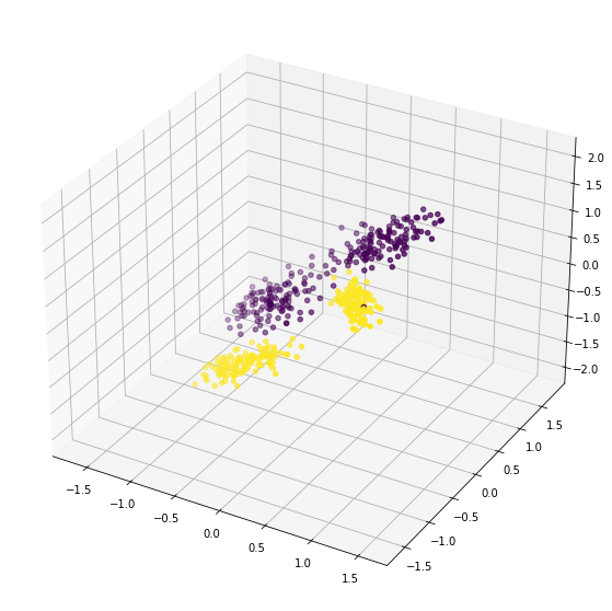
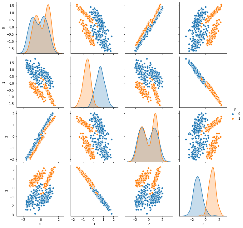
from sklearn.datasets import make_classification

X,y = make_classification(n_samples=500,n_features=4)
y = y.reshape(-1,1)
X.shape, y.shape
[7]:
((500, 4), (500, 1))
[8]:
df = pd.DataFrame(X)
df['y'] = y
df.head()
[8]:
| 0 | 1 | 2 | 3 | y | |
|---|---|---|---|---|---|
| 0 | -1.394862 | 1.068507 | -1.687573 | -1.411072 | 0 |
| 1 | 0.317359 | 1.075521 | 0.914416 | -1.940417 | 0 |
| 2 | -1.540031 | 1.312455 | -1.809805 | -1.785586 | 0 |
| 3 | -0.802099 | 1.197226 | -0.735972 | -1.810919 | 0 |
| 4 | -0.235792 | -0.109292 | -0.401901 | 0.258678 | 0 |
[9]:
%matplotlib inline
fig = plt.figure(figsize=(10,10))

ax = plt.axes(projection='3d')

ax.scatter(X[...,0],X[...,1],X[...,2],c=y)

plt.show()
[10]:
sns.pairplot(df,hue='y')
[10]:
<seaborn.axisgrid.PairGrid at 0x7f21a03bf9d0>
[11]:
from sklearn.metrics import confusion_matrix,accuracy_score
Logitsic Regression without Regularization#
Batch Gradient Descent#
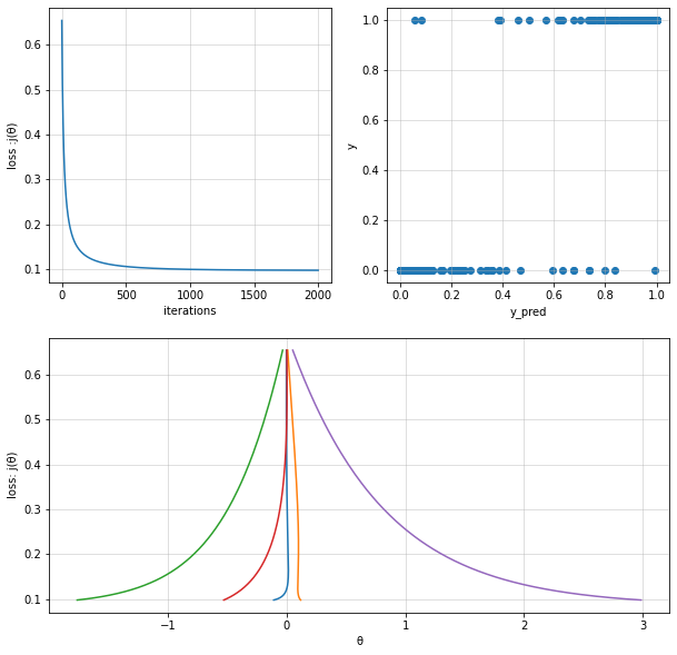
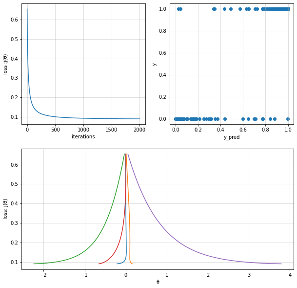
[31]:
logisitc_reg_model1 = LogisticRegression(alpha=0.1, iterations=2000)
logisitc_reg_model1.train(X=X, y=y, method="BGD", verbose=False)

y_pred = logisitc_reg_model1.predict(X)
theta = logisitc_reg_model1.theta
theta_history = logisitc_reg_model1.theta_history
cost_history = logisitc_reg_model1.cost_history


print("Fit theta :",theta)

print(f"""
Confusion Matrix :
{confusion_matrix(y,y_pred>0.5)}
Accuracy Score   :
{accuracy_score(y,y_pred>0.5)}
""")


fig = plt.figure(figsize=(10,10))
ax = fig.add_subplot(2,2,1)
ax.set(
    xlabel="iterations",
    ylabel="loss :j(θ)"
)
ax.plot(cost_history)
ax.grid(alpha=0.5)

ax = fig.add_subplot(2,2,2)
ax.set(
    xlabel="y_pred",
    ylabel="y"
)
ax.scatter(y_pred,y)
ax.grid(alpha=0.5)

ax = fig.add_subplot(2,2,(3,4))
ax.set(
    ylabel="loss: j(θ)",
    xlabel="θ"
)
ax.plot(theta_history,cost_history)
ax.grid(alpha=0.5)
plt.show()
Fit theta : [[-0.21130795  0.16250085 -2.23739897 -0.65426128  3.7890939 ]]

Confusion Matrix :
[[243   9]
 [  6 242]]
Accuracy Score   :
0.97
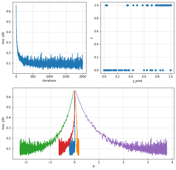
Stochastic Gradient Descent#
[22]:
logisitc_reg_model2 = LogisticRegression(alpha=0.1, iterations=2000)
logisitc_reg_model2.train(X=X, y=y, method="SGD",batch_size=200, verbose=False)

y_pred = logisitc_reg_model2.predict(X)
theta = logisitc_reg_model2.theta
theta_history = logisitc_reg_model2.theta_history
cost_history = logisitc_reg_model2.cost_history


print("Fit theta :",theta)

print(f"""
Confusion Matrix :
{confusion_matrix(y,y_pred>0.5)}
Accuracy Score   :
{accuracy_score(y,y_pred>0.5)}
""")


fig = plt.figure(figsize=(10,10))
ax = fig.add_subplot(2,2,1)
ax.set(
    xlabel="iterations",
    ylabel="loss :j(θ)"
)
ax.plot(cost_history)
ax.grid(alpha=0.5)

ax = fig.add_subplot(2,2,2)
ax.set(
    xlabel="y_pred",
    ylabel="y"
)
ax.scatter(y_pred,y)
ax.grid(alpha=0.5)

ax = fig.add_subplot(2,2,(3,4))
ax.set(
    ylabel="loss: j(θ)",
    xlabel="θ"
)
ax.plot(theta_history,cost_history)
ax.grid(alpha=0.5)
plt.show()
Fit theta : [[-0.2082787   0.17501482 -2.23356835 -0.63291115  3.77958104]]

Confusion Matrix :
[[243   9]
 [  6 242]]
Accuracy Score   :
0.97
Logistic Regression with Regularization#
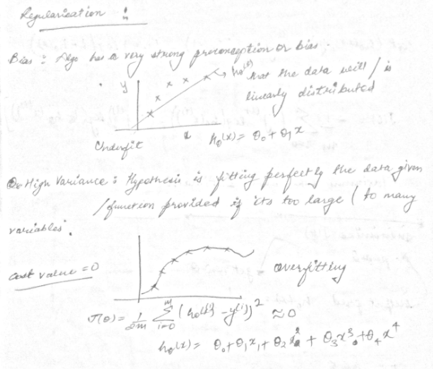
Addressing Overfitting
Reduce features
manually select
model selection algorithm
Regularization
Keep all the features but reduce magnitude/values of parameter theta
Works well when we have a lot of features and each contributes a bit to predicting y
\begin{align} \text{repeat until convergence \{}\\ \theta_0 &:= \theta_0 - \alpha \frac{1}{m} {\sum_{i=1}^{m} (h_{\theta}(x^{(i)}) - y^{(i)}) x_0^{(i)}}\\ \theta_j &:= \theta_j - \alpha \big[ \frac{1}{m} {\sum_{i=1}^{m} (h_{\theta}(x^{(i)}) - y^{(i)}) x_j^{(i)}} + \frac{\lambda}{m} {\theta_j} \big]\\ \text{\}\\}\\ \end{align}
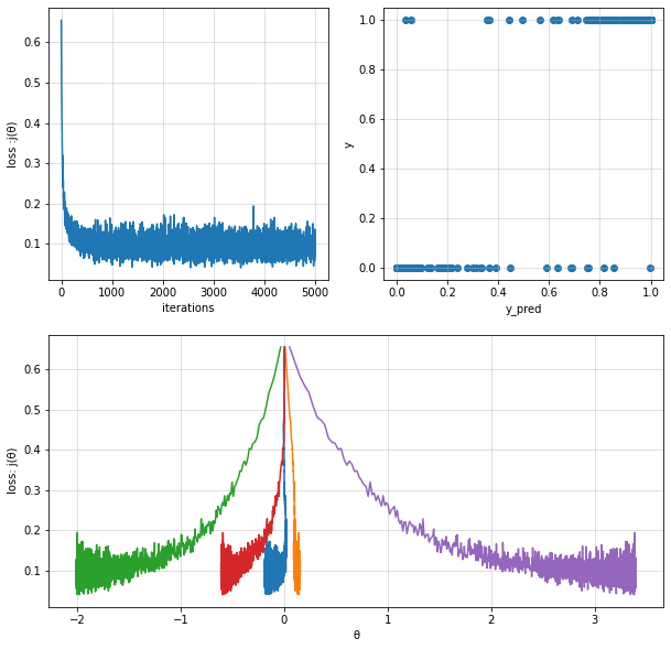
Stochastic Gradient Descent#
[29]:
logisitc_reg_model3 = LogisticRegression(alpha=0.1, iterations=5000)
logisitc_reg_model3.train(X=X, y=y, method="SGD",batch_size=300,regularization=True,penalty=1.0, verbose=False)

y_pred = logisitc_reg_model3.predict(X)
theta = logisitc_reg_model3.theta
theta_history = logisitc_reg_model3.theta_history
cost_history = logisitc_reg_model3.cost_history


print("Fit theta :",theta)

print(f"""
Confusion Matrix :
{confusion_matrix(y,y_pred>0.5)}
Accuracy Score   :
{accuracy_score(y,y_pred>0.5)}
""")


fig = plt.figure(figsize=(10,10))
ax = fig.add_subplot(2,2,1)
ax.set(
    xlabel="iterations",
    ylabel="loss :j(θ)"
)
ax.plot(cost_history)
ax.grid(alpha=0.5)

ax = fig.add_subplot(2,2,2)
ax.set(
    xlabel="y_pred",
    ylabel="y"
)
ax.scatter(y_pred,y)
ax.grid(alpha=0.5)

ax = fig.add_subplot(2,2,(3,4))
ax.set(
    ylabel="loss: j(θ)",
    xlabel="θ"
)
ax.plot(theta_history,cost_history)
ax.grid(alpha=0.5)
plt.show()
Fit theta : [[-0.17386854  0.13890258 -1.98945975 -0.58958285  3.37052331]]

Confusion Matrix :
[[243   9]
 [  6 242]]
Accuracy Score   :
0.97
Batch Gradient Descent#
[24]:
logisitc_reg_model4 = LogisticRegression(alpha=0.1, iterations=2000)
logisitc_reg_model4.train(X=X, y=y, method="BGD", regularization=True, penalty=2.0, verbose=False)

y_pred = logisitc_reg_model4.predict(X)
theta = logisitc_reg_model4.theta
theta_history = logisitc_reg_model4.theta_history
cost_history = logisitc_reg_model4.cost_history


print("Fit theta :",theta)

print(f"""
Confusion Matrix :
{confusion_matrix(y,y_pred>0.5)}
Accuracy Score   :
{accuracy_score(y,y_pred>0.5)}
""")


fig = plt.figure(figsize=(10,10))
ax = fig.add_subplot(2,2,1)
ax.set(
    xlabel="iterations",
    ylabel="loss :j(θ)"
)
ax.plot(cost_history)
ax.grid(alpha=0.5)

ax = fig.add_subplot(2,2,2)
ax.set(
    xlabel="y_pred",
    ylabel="y"
)
ax.scatter(y_pred,y)
ax.grid(alpha=0.5)

ax = fig.add_subplot(2,2,(3,4))
ax.set(
    ylabel="loss: j(θ)",
    xlabel="θ"
)
ax.plot(theta_history,cost_history)
ax.grid(alpha=0.5)
plt.show()
Fit theta : [[-0.10691344  0.11932182 -1.76102026 -0.52738503  2.98468473]]

Confusion Matrix :
[[243   9]
 [  5 243]]
Accuracy Score   :
0.972