
Probability Estimation (MLE & MAP)#
References#
https://www.cs.cornell.edu/courses/cs4780/2018fa/lectures/lecturenote04.html
https://www.cs.cornell.edu/courses/cs4780/2018fa/lectures/lecturenote05.html
[1]:
import numpy as np
import pandas as pd

import matplotlib.pyplot as plt
import seaborn as sns

plt.style.use('fivethirtyeight')
Intro#
P(X, Y) distribution P of data X & Y.
When we estimate P(X, Y) = P(X|Y) P(Y) = P(Y|X) P(X), called Generative Learning.
When we only estimate P(Y|X) directly, called Discriminative Learning.
Scenario Coin Toss
Probability of getting heads P(H), when the coin is not a perfect one?
number of tosses = 10
10 samples are collected from tosses, D = { H, H, T, T, H, T, H, T, T, T }
here \(n_H\) = 4 and \(n_T\) = 6, hence
\(P(H) \approx \frac{n_H}{n_H + n_T} = \frac{4}{4 + 6} = 0.4\)
lets try to derive it…
Maximum Likelihood Estimation(MLE)#
Estimation mentioned above in the scenario is actually Maximum Likelihood Estimation. P(H) is estimation of likelihood of getting heads.
Steps for MLE-
Modeling assumption about the type of distribution data is coming from.
fitting the distribution parameter so that the sample/data observed is likely as possible.
for coin toss example the distribution observed is binomial distribution {0, 1}. binom distribution has two parameters n and \(\theta\).
\begin{align} b(x;n,\theta) &= \binom{n}{x}{\theta^x}{(1-\theta)}^{(n-x)}\\ \\ where \\ n &= \text{number of random events}\\ \theta &= \text{probability of the event x} \end{align}
in the scenario’s context
\begin{align} P(D;\theta) &= \binom{n_H + n_T}{n_H}{\theta^{n_H}}{(1-\theta)}^{(n-n_H)}\\ \\ where \\ n &= \text{number of independent bernoulli(binary) random events}\\ \theta &= \text{probability of heads coming up} = P(H) \end{align}
This translates to find a distribution \(P(D|\theta)\) which has two parameters n and \(\theta\) and it captures the distribution of n independent bernoulli random events(that generates random 0 and 1 ) such that \(\theta\) is the probability of the coin coming up with heads.
Principle
find \(\hat{\theta}\) to maximize the likelihood of the data, \(P(D;\theta)\):
\(\hat{\theta}_{MLE} = {argmax\atop{\theta}} P(D; \theta)\)
to maximize the value from a equation generally the derivative of the equation is solved while equating it to 0.
two steps to solve above equation
apply log to the function (In computer science we dont prefer multiplying probabilities due to muliple reasons(see reference section). Hence we take log and convert multiplication to addition.)
calculate derivative of equation and equate it to 0.
\begin{align} \hat{\theta}_{MLE} &= {argmax\atop{\theta}} P(D; \theta)\\ &= {argmax\atop{\theta}} \binom{n_H + n_T}{n_H}{\theta^{n_H}}{(1-\theta)}^{(n_T)}\\ &= {argmax\atop{\theta}} \log{[ \binom{n_H + n_T}{n_H}{\theta^{n_H}}{(1-\theta)}^{(n_T)}]}\\ &= {argmax\atop{\theta}} \log{[ \binom{n_H + n_T}{n_H} ]} + \log{[\theta^{n_H}]} + \log{[(1-\theta)^{n_T}]}\\ &\downarrow \frac{\partial}{\partial \theta}\text{ calculate derivative}\\ \frac{n_H}{\theta} + \frac{n_T}{1 - \theta} &= 0\\ \hat{\theta} &= \frac{n_H}{n_H + n_T}\\ \\ \text{where } \theta \in [0, 1] \end{align}
[2]:
np.random.seed(0)
[3]:
events = [ "T", "H" ]

n_events = 50
D = np.random.choice(events, n_events)

D
[3]:
array(['T', 'H', 'H', 'T', 'H', 'H', 'H', 'H', 'H', 'H', 'H', 'T', 'T',
       'H', 'T', 'T', 'T', 'T', 'T', 'H', 'T', 'H', 'H', 'T', 'T', 'H',
       'H', 'H', 'H', 'T', 'H', 'T', 'H', 'T', 'H', 'H', 'T', 'H', 'H',
       'T', 'T', 'H', 'T', 'H', 'H', 'H', 'H', 'H', 'T', 'H'], dtype='<U1')
[4]:
from scipy.stats import binom
[5]:
n = dict(zip(*np.unique(D, return_counts=True)))
n
[5]:
{'H': 30, 'T': 20}
[6]:
theta = n['H']/(n['H'] + n['T'])
theta
[6]:
0.6
[7]:
binom_distribution = binom(n=n_events, p=theta)
[8]:
x = np.arange(binom_distribution.ppf(0.01), binom_distribution.ppf(0.99))
[9]:
fig, ax = plt.subplots(1, 2, figsize=(10, 5))

ax[0].plot(x, binom_distribution.pmf(x), 'ko', label='pmf')
# ax[0].plot(x, binom_distribution.cdf(x), '--', label='cdf')
ax[0].vlines(x, 0, binom_distribution.pmf(x), colors='b', lw=5, alpha=0.5)
ax[0].legend()

ax[1].hist(binom_distribution.rvs(1000), label='rvs', edgecolor='white', bins=10, density=False)
ax[1].legend()

plt.show()
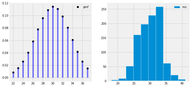
Likelihood of getting 56 heads in 100 coin toss trials have the highest probability with 56% success rate. Hence the above plot represents maximum likelihood estimation of getting a head(success event) out of 100 trials with success rate of 56%, number of successes on x axis and probability of success on y axis.
[10]:
theta
[10]:
0.6
This could be unreasonable, when
we only have heads, less number of observations(less data)
easily can overfit if data is not enough
Scenario coin toss with prior knowledge
Lets assume we already know that the \(\theta\) should be close to 0.5, and the size of sample is small.
To fix the results we can
\begin{align*} \hat{\theta} &= \frac{n_H + m}{n_H + n_T + 2m} \end{align*}
m = number of heads/tails to the data, as prior belief, that these are pseudo trials already done and obsevations are added directly.
[11]:
for m in range(0, 101, 10):
    theta = (n['H'] + m)/(n['H'] + n['T'] + 2*m)
    print("m :", m, " theta :", theta)
m : 0  theta : 0.6
m : 10  theta : 0.5714285714285714
m : 20  theta : 0.5555555555555556
m : 30  theta : 0.5454545454545454
m : 40  theta : 0.5384615384615384
m : 50  theta : 0.5333333333333333
m : 60  theta : 0.5294117647058824
m : 70  theta : 0.5263157894736842
m : 80  theta : 0.5238095238095238
m : 90  theta : 0.5217391304347826
m : 100  theta : 0.52
if n is too large, then this change will be insignificant but for smaller n it will drive the results closer to our hunch. It is called smoothing. We will derive formally in next topics.
Naive Bayes#
\begin{align} P(Y=y | X=x) &= \frac{P(X=x | Y=y) P(Y=y)}{P(X=x)}\\ \\ &\text{Where } \\ P(X=x | Y=y) &= \prod_{\alpha=1}^{d} P([X]_\alpha = x_\alpha| Y = y) \end{align}
Naively assumes that all the features used are independently distrubuted variables given the label Y.
for example given that there is an email where all the words are independent given the label spam/ham.
Bayes Classifier#
\begin{align*} h(\vec{x}) &= {argmax\atop{y}} \frac{P(\vec{x} | y) P(y)}{z}\\ \\ &= {argmax\atop{y}} P(y) \prod_{\alpha} P([\vec{X}]_\alpha | y)\\ \\ &= {argmax\atop{y}} ( log(P(y) + \sum_\alpha log P([\vec{X}]_\alpha | y)) \end{align*}
P.S. - In computer science we dont prefer multiplying probabilities due to muliple reasons(see reference section). Hence we take log and convert multiplication to addition.
The Bayesian Way#
In bayesian statistics we can consider \(\theta\) is a random variable, drawn from \(P(\theta)\), and IT IS NOT ASSOCIATED WITH AN EVENT FROM SAMPLE SPACE. We can’t do that in frequentist statistics. Hence in bayesian statistics we are allowed to have prior belief about \(\theta\).
From Bayes rule we can look at
\begin{align*} & P(\theta | D) = \frac{P(D | \theta)p(\theta)}{p(D)}\\ \end{align*}
where
\(P(\theta)\) is the prior knowledge, prior distribution over the parameter \(\theta\), before we see any data.
\(P(D | \theta)\) is the likelihood of the data given the parameter \(\theta\).
\(P(\theta | D)\) is the posterior distribution over the parameter \(\theta\), after we have observed the data.
\begin{align*} P(\theta) &= \frac{\theta^{\alpha - 1} (1 - \theta)^{\beta - 1}}{B(\alpha, \beta)}\\ \\ P(\theta | D) &\propto P(D | \theta) P(\theta)\\ P(\theta | D) &\propto \binom{n_H + n_T}{n_H} \theta^{n_H} (1 - \theta)^{n_T} \theta^{\alpha - 1} ( 1 - \theta)^{\beta - 1} \end{align*}
Maximum A Posteriori Probability Estimation(MAP)#
MAP Principle : find \(\hat{\theta}\) that maximinzes the posterior distribution \(P(\theta | D)\)
\begin{align} \hat{\theta} &= {argmax\atop{\theta}} P(\theta | D)\\ \hat{\theta} &= {argmax\atop{\theta}} \binom{n_H + n_T}{n_H} \theta^{n_H} (1 - \theta)^{n_T} \theta^{\alpha - 1} ( 1 - \theta)^{\beta - 1}\\ &\downarrow \text{ apply log and }\frac{\partial}{\partial \theta}\\ &= {argmax\atop{\theta}} n_H \log(\theta) + n_T \log(1 - \theta) + (\alpha - 1) \log(\theta) + (\beta - 1) \log(1 - \theta) \\ &=\frac{n_H + \alpha - 1}{n_H + n_T + (\alpha - 1) + (\beta - 1)} \end{align}
Please Note -
MLE and MAP are identical with \(\alpha - 1\) hallucinated heads and \(\beta - 1\) hallucinated tails, that translates to our prior beiefs
if n is really large then MAP becomes MLE, \(\alpha - 1\) and \(\beta - 1\) become irrelevant compared to large \(n_H\) and \(n_T\)
MAP can be a really great esitmator if tf prior belief is available and accurate
if n is small, then MAP can be wrong if prior belief is not accurate.
in essence \(\alpha - 1\) and \(\beta - 1\) are corrections based on prior expertise/ belief/ knowledge in the results of probabiliy estimation if n is small. these corrections are based on situational assumptions and can be wrong if assumptions do not match.
Bayesian Statisics vs Frequentist Statisitcs#
Connecting this to ML#
In supervised ML we are provided with data D, we train the model with its parameters \(\theta\), this model is used to generate predictions for \(x_t\)
MLE : \(P(y|x_t ; \theta) \rightarrow \text{ Learning }\theta = argmax_{\theta} P(D; \theta)\), \(\theta\) is purely a model parameter.
MAP : \(P(y|x_t ; \theta) \rightarrow \text{ Learning }\theta = argmax_{\theta} P(\theta | D) \propto P(D | \theta)P(\theta)\), Here \(\theta\) is a random variable.
True Bayesian Approach : \(P(y|X=x_t) = \int_{0}^{\theta} P(y| \theta) p(\theta | D) d\theta\) , our prediction takes all possible models into account.