Linear Regression

References

• https://www.youtube.com/watch?v=xpHQ6UhMlx4

Intro

• linear regression, a very simple approach for supervised learning. In particular, linear regression is a useful tool for predicting a quantitative response.

• In statistics, linear regression is a linear approach to modelling the relationship between a scalar response and one or more explanatory variables (also known as dependent and independent variables).

• The case of one explanatory variable is called simple linear regression; for more than one, the process is called multiple linear regression.

                training-set
                    |
                    V
            Learning algorithm
                    |
                    V
            +-------------+
test -->    | hypothesis  | --> estimation
            |    / Model  |
            +-------------+

\begin{align} \text{Hypothesis } h_\theta(x) &= \theta_0 + \theta_1 x \text{, Where Parameters } : \theta_0, \theta_1 \end{align}

\begin{align} \text{Cost Function } &: J(\theta_0,\theta_1) = \frac{1}{2m}\sum_{i=1}^{m}(h_\theta{(x^{(i)}) - y^{(i)}})^2\\ \\ \text{Goal} &: {{minimize}\atop{\theta_0,\theta_1}} J(\theta_0,\theta_1) \end{align}

Generate Data

import pandas as pd
import numpy as np
from sklearn.datasets import make_regression
import matplotlib.pyplot as plt
from mpl_toolkits import mplot3d
import seaborn as sns

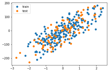
sample_size = 300
train_size = 0.7 # 70%

X, y = make_regression(n_samples=sample_size, n_features=1, noise=50,random_state=0)
y = y.reshape(-1,1)


np.random.seed(10)
random_idxs = np.random.permutation(np.arange(0, sample_size))[: int(np.ceil(sample_size * train_size))]

X_train, y_train = X[random_idxs], y[random_idxs]
X_test, y_test = np.delete(X, random_idxs).reshape(-1, 1), np.delete(y, random_idxs).reshape(-1, 1)

plt.plot(X_train, y_train, 'o', label='train')
plt.plot(X_test, y_test, 'o', label='test')
plt.legend()
plt.show()

• X = (m,n), where

  m = number of samples

  n = number of features

• Add \(X_0\) (column 0 as 1) for bias in linear regression \begin{align} h_\theta(x) &= \theta_0 X_0 + \theta_1 X_1 \\ \because X_0 &= 1 \\ h_\theta(x) &= \theta_0 + \theta_1 X_1 \\ \end{align}

print(X.shape, y.shape)

(300, 1) (300, 1)

m, n = X.shape
print("number of columns (features) :",n)
print("number of samples (rows) :",m)

number of columns (features) : 1
number of samples (rows) : 300

def add_axis_for_bias(X_i):

    X_i = X_i.copy()
    if len(X_i.shape) == 1:
        X_i = X_i.reshape(-1,1)

    if False in (X_i[...,0] == 1):
        return np.hstack(tup=(np.ones(shape=(X_i.shape[0],1)) , X_i))
    else:
        return X_i

Check for bias column(column 0)

arr = np.array([
    [1,2,3,4],
    [1,6,7,8],
    [1,11,12,13],
    [1,4,2,4],
    [1,5,2,1],
    [1,7,54,23]
])

arr.shape

(6, 4)

• this means 6 rows and 4 columns

False not in (arr[...,0] == 1)

True

np.sum(arr), np.sum(arr, axis=0), np.sum(arr, axis=1)

(174, array([ 6, 35, 80, 53]), array([10, 22, 37, 11,  9, 85]))

np.mean(arr), np.mean(arr,axis=0), np.mean(arr, axis=1)

(7.25,
 array([ 1.        ,  5.83333333, 13.33333333,  8.83333333]),
 array([ 2.5 ,  5.5 ,  9.25,  2.75,  2.25, 21.25]))

for us calculation will be done column wise so axis = 0 everywhere

Regression Models Error Evaluation Functions

Mean Squared Error

def calculate_mse(y_pred,y):
    return np.square(y_pred - y).mean()

Root Mean Squared Error

def calculate_rmse(y_pred,y):
    return np.sqrt(np.square(y_pred - y).mean())

Mean Absolute Error

def calculate_mae(y_pred,y):
    return np.abs(y_pred - y).mean()

Algorithm

Cost Function

\begin{align} J(\theta_0,\theta_1) & =\frac{1}{2m}\sum_{i=1}^{m}({h_\theta{(x^{(i)}) - y^{(i)}}})^2 \end{align}

def calculate_cost(y_pred,y):
    return np.mean(np.square(y_pred - y)) / 2

Derivative

\begin{align} \frac{\partial J(\theta_0,\theta_1)}{\partial \theta} &= \frac{1}{m} \sum_{i=1}^{m}(h_{\theta}(x^{(i)}) - y^{(i)}). x^{(i)} \end{align}

def derivative(X, y, y_pred):
    return np.mean( ( y_pred - y ) * X, axis = 0 )

Gradient Descent Algorithm

\begin{align} \text{repeat until convergence } \{ \\ \theta_j &:= \theta_j - \alpha \frac{\partial}{\partial\theta_j}{J(\theta_0,\theta_1)}\\ \}\text{ for j=0 and j=1 }\\ \\ \text{and simultaneously update }\\ temp_0 &:= \theta_0 - \alpha\frac{\partial}{\partial\theta_0}{J(\theta_0,\theta_1)}\\ temp_1 &:= \theta_1 - \alpha\frac{\partial}{\partial\theta_1}{J(\theta_0,\theta_1)}\\ \theta_0 &:= temp_0\\ \theta_1 &:= temp_1 \end{align}

Final algorithm

\begin{align} \text{repeat until convergence }\{\\ \theta_0 &:= \theta_0 - \alpha \frac{1}{m}{\sum_{i=1}^{m}{(h_\theta(x^{(i)}) - y^{(i)})}}\\ \theta_1 &:= \theta_1 - \alpha \frac{1}{m}{\sum_{i=1}^{m}{(h_\theta(x^{(i)}) - y^{(i)})}}.{x^{(i)}}\\ \} \end{align}

Generate Prediction

def predict(theta,X):
    format_X = add_axis_for_bias(X)

    if format_X.shape[1] == theta.shape[0]:
        y_pred = format_X @ theta # (m,1) = (m,n) * (n,1)
        return y_pred
    elif format_X.shape[1] == theta.shape[1]:
        y_pred = format_X @ theta.T # (m,1) = (m,n) * (n,1)
        return y_pred
    else:
        raise ValueError("Shape is not proper.")

Batch Gradient Descent

def linear_regression_bgd(X, y, verbose = True, theta_precision = 0.001, alpha = 0.01, iterations = 10000):
    X = add_axis_for_bias(X)

    # number of features+1 because of theta_0
    m, n = X.shape

    theta_history = []
    cost_history = []

    theta = np.random.rand(1,n) * theta_precision

    for iteration in range(iterations):
        # calculate y_pred
        theta_history.append(theta[0])

        y_pred = predict(theta,X)

        # simultaneous operation
        gradient = derivative(X, y, y_pred)

        theta = theta - (alpha *  gradient) # override with new θ

        if np.isnan(np.sum(theta)) or np.isinf(np.sum(theta)):
            print("breaking. found inf or nan.")
            break

        # calculate cost to put in history
        cost = calculate_cost(predict(theta, X), y)

        cost_history.append(cost)

    return theta, np.array(theta_history), np.array(cost_history)

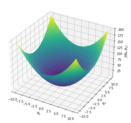
Cost function vs weights \(J(\theta_0, \theta_1)\)

theta0,theta1 = np.meshgrid(np.linspace(-10,10,100),np.linspace(-10,10,100))
j = theta0**2 + theta1**2

fig = plt.figure(figsize=(7,7))
ax = plt.axes(projection='3d')

ax.plot_surface(theta0, theta1, j, cmap='viridis')
ax.set_xlabel('$\\theta_0$')
ax.set_ylabel('$\\theta_1$')
ax.set_zlabel('$J(\\theta_0,\\theta_1)$')

plt.show()

Debugging gradient descent

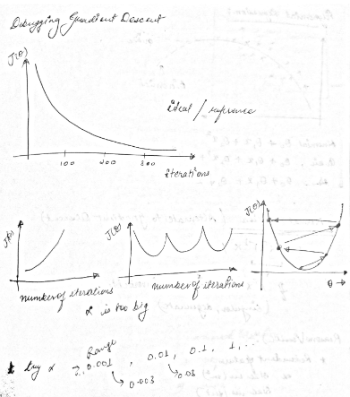
if learning rate is high, theta value will increase too much and eventually shoot out of the plot. see an example below.

if learning rate is appropriate then value of cost/loss will decrease and eventually flatlines (decrement is too less to matter). see an example below

we can try different learning rate like 0.001, 0.003, 0.01, 0.03, 0.1 etc.

Animation Function

from utility import regression_animation

Training with high learning rate

iterations = 600
learning_rate = 2.03

theta, theta_history, cost_history = linear_regression_bgd(X_train, y_train, verbose=True, theta_precision = 0.001,
                                                           alpha = learning_rate ,iterations = iterations)

regression_animation(X_train, y_train, cost_history, theta_history, iterations, interval=10)

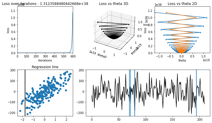
learning rate is high, model couldn’t converge(find minima in loss-theta curve), hence :math:`J(theta_0, theta_1)` increased.

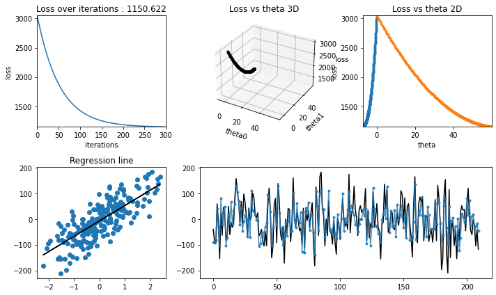
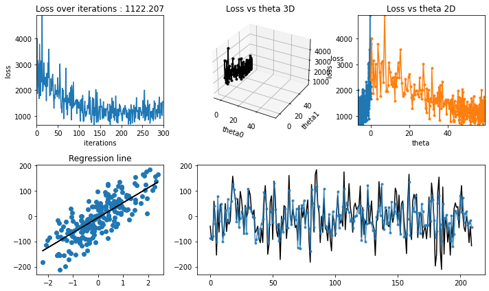
Training with learning rate = 0.01

iterations = 300
learning_rate = 0.01

theta, theta_history, cost_history = linear_regression_bgd(X_train, y_train, verbose=True, theta_precision = 0.001,
                                                           alpha = learning_rate ,iterations = iterations)

regression_animation(X_train, y_train, cost_history, theta_history, iterations, interval=10)

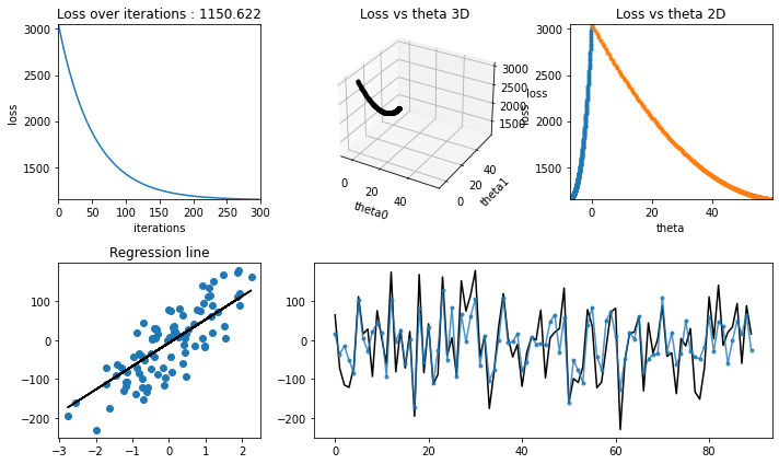
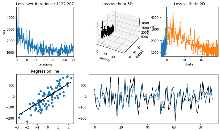
Testing

regression_animation(X_test, y_test, cost_history, theta_history, iterations, interval=10)

Stochastic gradient Descent

• Stochastic gradient descent (often abbreviated SGD) is an iterative method for optimizing an objective function with suitable smoothness properties (e.g. differentiable or subdifferentiable).

• It can be regarded as a stochastic approximation of gradient descent optimization, since it replaces the actual gradient (calculated from the entire data set) by an estimate thereof (calculated from a randomly selected subset of the data).

• Especially in high-dimensional optimization problems this reduces the computational burden, achieving faster iterations in trade for a lower convergence rate.

It is - an iterative method - train over random samples of a batch size instead of training on whole dataset - faster convergence on large dataset

def linear_regression_sgd(X, y, verbose=True, theta_precision = 0.001, batch_size=30,
                          alpha = 0.01 ,iterations = 10000):
    X = add_axis_for_bias(X)

    # number of features+1 because of theta_0
    m, n = X.shape

    theta_history = []
    cost_history = []

    theta = np.random.rand(1,n) * theta_precision

    for iteration in range(iterations):

        theta_history.append(theta[0])

        # creating indices for batches
        indices = np.random.randint(0, m, size=batch_size)

        # creating batch for this iteration
        X_rand = X[indices]
        y_rand = y[indices]

        y_pred = predict(theta, X_rand)

        # simultaneous operation
        gradient = derivative(X_rand, y_rand, y_pred)
        theta = theta - (alpha *  gradient)

        if np.isnan(np.sum(theta)) or np.isinf(np.sum(theta)):
            print("breaking. found inf or nan.")
            break

        # calculate cost to put in history
        cost = calculate_cost(predict(theta, X_rand), y_rand)
        cost_history.append(cost)

        # calcualted theta in history
    return theta, np.array(theta_history), np.array(cost_history)

Training for learning rate = 0.01

iterations = 300
learning_rate = 0.01

theta, theta_history, cost_history = linear_regression_sgd(X_train, y_train, verbose=True, theta_precision = 0.001,
                                                           alpha = learning_rate ,iterations = iterations)

regression_animation(X_train, y_train, cost_history,theta_history, iterations, interval=10)

regression_animation(X_test, y_test, cost_history,theta_history, iterations, interval=10)

Normal Equation (Closed Form)

normal equation vs gradient descent

Gradient Descent	Normal Equation
Need to choose learning rate alpha	no need to choose alpha
needs iteration	doesn’t need iterations
works well with large number of features ( n large )	computation increases for large n
feature scaling will help in convergence	no need to do feature scaling

Derivation

\begin{align} L(\theta) &= \frac{1}{n} \sum_{i=0}^{n-1} (\theta^T x - y)^2\\ \\ &\text{where } \vec{x}: (m \times n) \quad \vec{y}: (m \times 1) \quad \vec{\theta}: (n \times 1)\\ \\ \text{lets take matrix form } (X \theta - y)^2 &= (X \theta - y)^T (X \theta - y)\\ \\ (X \theta - y)^2 &= \theta^T X^T X \theta - \theta^T X^T y - y^T X \theta - y^T y\\ \\ \because \theta^T X^T y : (1 \times n)(n \times m)(m \times 1) = (1 \times 1) = \text{scalar value}\\ \\ \text{and } y^T X \theta : (1 \times m)(m \times n)(n \times 1) = (1 \times 1) = \text{scalar value}\\ \\ \text{and } a^T b = b^T a \text{ for scalar value}\\ \\ \therefore (X \theta - y)^2 &= \theta^T X^T X \theta - 2 \theta^T X^T y - y^T y\\ \\ \text{to find minima equating dervative of } \theta \text{ to zero}\\ \\ \frac{\delta L}{\delta \theta} &= 0\\ \\ 2 X^T X \theta - 2 X^T y &= 0\\ \\ X^T X \theta &= X^T y\\ \\ \theta &= (X^T X)^{-1} X^T y \end{align}

def linear_regression_normaleq(X, y):
    X = add_axis_for_bias(X)
    theta = np.linalg.inv(X.T @ X) @ X.T @ y
    return theta

theta = linear_regression_normaleq(X_train, y_train)

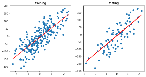
fig, ax = plt.subplots(1,2, figsize=(10, 5))

y_pred = predict(theta, X_train)

ax[0].scatter(X_train, y_train)
ax[0].plot(X_train, y_pred, c='r')
ax[0].set_title("training")

y_pred = predict(theta, X_test)

ax[1].scatter(X_test, y_test)
ax[1].plot(X_test,y_pred,c='r')
ax[1].set_title("testing")

plt.show()