
Statsmodels#
Mathematical equation which explains the relationship between dependent variable (Y) and independent variable(X).
Y = f(X)
Due to uncertainy in result and noise the equation is
Y = f(X) + e
Linear Models#
\begin{align} Y &= \theta_0 + \theta_1 X_1 + \theta_2 X_2 + ... + \theta_n X_n\\ Y &= \theta_0 + \theta_1 X + \theta_2 X^2 + ... + \theta_n X^n\\ Y &= \theta_0 + \theta_1 sin(X_1) + \theta_2 * cos(X_2) \end{align}
Linear Regression#
\begin{align} Y &= \theta_0 + \theta_1 * X + e\\ & \theta_0, \theta_1 = Coefficient\\ & e = normally distributed residual error \end{align}
Linear Regression model assumes that residuals are independent and normally distributed
Model is fitted to the data using ordinary least squares approach
Non-Linear Models#
Most of the cases, the non-linear models are generalized to linear models
Binomial Regresson, Poisson Regression
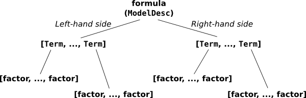
Design Matrices#
Once the model is chosen design metrices are constructed. Y = XB + e
Variable |
Description |
|---|---|
Y |
vector/matrix of dependent variable |
X |
vector/matrix of independent variable |
B |
vector/matrix of coefficient |
e |
residual error |
Creating a Model#
using statsmodel library#
OLS (oridinart least squares)
GLM (genralized linear model)
WLS (weighted least squares)
ols
glm
wls
Uppercase names take design metrices as args
Lowercase names take Patsy formulas and dataframes as args
Fitting a Model#
fitting method returns a model object for futher methods, attributes and coefficient matrix for analysis
View Model Summary#
Describe the fit description of the model in text.
Construct Design Matrices#
\(Y = \theta_0 + \theta_1 X_1 + \theta_2 X_2 + \theta_3 X_1 X_2\)
Design Matrix with Numpy#
[1]:
import numpy as np

Y = np.array([1,2,3,4,5]).reshape(-1,1)

x1 = np.array([6,7,8,9,10])
x2 = np.array([11,12,13,14,15])

X = np.vstack([np.ones(5), x1, x2, x1*x2]).T

print(Y)
print(X)
[[1]
 [2]
 [3]
 [4]
 [5]]
[[  1.   6.  11.  66.]
 [  1.   7.  12.  84.]
 [  1.   8.  13. 104.]
 [  1.   9.  14. 126.]
 [  1.  10.  15. 150.]]
Design Matrix with patsy#
allows defining a model easily
constructs relevant design matrices (patsy.dmatrices)
takes a formula in string form as arg and a dictionary like object with data arrays for resoponse variables
    ~
 /    \
Y     +
    /   \
   1     +
       /   \
      x1    +
          /   \
        x2     *
             /   \
           x1    x2
‘y ~ np.log(x1)’: Often numpy functions can be used to transform terms in the expression.
‘y ~ I(x1 + x2)’: I is the identify function, used to escape arithmetic expressions and are evaluated.
‘y ~ C(x1)’: Treats the variable x1 as a categorical variable.
[2]:
import patsy

y = np.array([1, 2, 3, 4, 5])
x1 = np.array([6, 7, 8, 9, 10])
x2 = np.array([11, 12, 13, 14, 15])
data = {
    'Y' : Y,
    'x1' : x1,
    'x2' : x2,
}

equation = 'Y ~ 1 + x1 + x2 + x1*x2'

Y, X = patsy.dmatrices(equation, data)

print(Y)
print(X)
[[1.]
 [2.]
 [3.]
 [4.]
 [5.]]
[[  1.   6.  11.  66.]
 [  1.   7.  12.  84.]
 [  1.   8.  13. 104.]
 [  1.   9.  14. 126.]
 [  1.  10.  15. 150.]]
load popular datasets from statsmodels#
[3]:
import statsmodels.api as sm
dataset = sm.datasets.cancer.load()
# dataset = sm.datasets.cancer.load_pandas()
dataset
[3]:
<class 'statsmodels.datasets.utils.Dataset'>
Linear Model Creation using statsmodels#
Using inbuilt Icecream dataset#
[4]:
import statsmodels.api as sm

icecream = sm.datasets.get_rdataset("Icecream","Ecdat")

dataset = icecream.data
dataset.head()
[4]:
| cons | income | price | temp | |
|---|---|---|---|---|
| 0 | 0.386 | 78 | 0.270 | 41 |
| 1 | 0.374 | 79 | 0.282 | 56 |
| 2 | 0.393 | 81 | 0.277 | 63 |
| 3 | 0.425 | 80 | 0.280 | 68 |
| 4 | 0.406 | 76 | 0.272 | 69 |
[5]:
import statsmodels.formula.api as smf

linearModel1 = smf.ols('cons ~ price + temp',dataset)

fitModel1 = linearModel1.fit()

print(fitModel1.summary())
                            OLS Regression Results
==============================================================================
Dep. Variable:                   cons   R-squared:                       0.633
Model:                            OLS   Adj. R-squared:                  0.606
Method:                 Least Squares   F-statistic:                     23.27
Date:                Thu, 15 Oct 2020   Prob (F-statistic):           1.34e-06
Time:                        21:53:43   Log-Likelihood:                 54.607
No. Observations:                  30   AIC:                            -103.2
Df Residuals:                      27   BIC:                            -99.01
Df Model:                           2
Covariance Type:            nonrobust
==============================================================================
                 coef    std err          t      P>|t|      [0.025      0.975]
------------------------------------------------------------------------------
Intercept      0.5966      0.258      2.309      0.029       0.067       1.127
price         -1.4018      0.925     -1.515      0.141      -3.300       0.496
temp           0.0030      0.000      6.448      0.000       0.002       0.004
==============================================================================
Omnibus:                        0.991   Durbin-Watson:                   0.656
Prob(Omnibus):                  0.609   Jarque-Bera (JB):                0.220
Skew:                          -0.107   Prob(JB):                        0.896
Kurtosis:                       3.361   Cond. No.                     6.58e+03
==============================================================================

Warnings:
[1] Standard Errors assume that the covariance matrix of the errors is correctly specified.
[2] The condition number is large, 6.58e+03. This might indicate that there are
strong multicollinearity or other numerical problems.
[6]:
linearModel2 = smf.ols('cons ~ income + temp',dataset)

fitModel2 = linearModel2.fit()

print(fitModel2.summary())
                            OLS Regression Results
==============================================================================
Dep. Variable:                   cons   R-squared:                       0.702
Model:                            OLS   Adj. R-squared:                  0.680
Method:                 Least Squares   F-statistic:                     31.81
Date:                Thu, 15 Oct 2020   Prob (F-statistic):           7.96e-08
Time:                        21:53:43   Log-Likelihood:                 57.742
No. Observations:                  30   AIC:                            -109.5
Df Residuals:                      27   BIC:                            -105.3
Df Model:                           2
Covariance Type:            nonrobust
==============================================================================
                 coef    std err          t      P>|t|      [0.025      0.975]
------------------------------------------------------------------------------
Intercept     -0.1132      0.108     -1.045      0.305      -0.335       0.109
income         0.0035      0.001      3.017      0.006       0.001       0.006
temp           0.0035      0.000      7.963      0.000       0.003       0.004
==============================================================================
Omnibus:                        2.264   Durbin-Watson:                   1.003
Prob(Omnibus):                  0.322   Jarque-Bera (JB):                1.094
Skew:                           0.386   Prob(JB):                        0.579
Kurtosis:                       3.528   Cond. No.                     1.56e+03
==============================================================================

Warnings:
[1] Standard Errors assume that the covariance matrix of the errors is correctly specified.
[2] The condition number is large, 1.56e+03. This might indicate that there are
strong multicollinearity or other numerical problems.
[7]:
linearModel3 = smf.ols('cons ~ -1 + income + temp',dataset)

fitModel3 = linearModel3.fit()

print(fitModel3.summary())
                                 OLS Regression Results
=======================================================================================
Dep. Variable:                   cons   R-squared (uncentered):                   0.990
Model:                            OLS   Adj. R-squared (uncentered):              0.990
Method:                 Least Squares   F-statistic:                              1426.
Date:                Thu, 15 Oct 2020   Prob (F-statistic):                    6.77e-29
Time:                        21:53:43   Log-Likelihood:                          57.146
No. Observations:                  30   AIC:                                     -110.3
Df Residuals:                      28   BIC:                                     -107.5
Df Model:                           2
Covariance Type:            nonrobust
==============================================================================
                 coef    std err          t      P>|t|      [0.025      0.975]
------------------------------------------------------------------------------
income         0.0023      0.000      9.906      0.000       0.002       0.003
temp           0.0033      0.000      8.571      0.000       0.003       0.004
==============================================================================
Omnibus:                        3.584   Durbin-Watson:                   0.887
Prob(Omnibus):                  0.167   Jarque-Bera (JB):                2.089
Skew:                           0.508   Prob(JB):                        0.352
Kurtosis:                       3.798   Cond. No.                         6.45
==============================================================================

Warnings:
[1] Standard Errors assume that the covariance matrix of the errors is correctly specified.
[8]:
import statsmodels.api as sm
import statsmodels.formula.api as smf
import numpy as np
df = sm.datasets.get_rdataset("mtcars").data


model = smf.ols('np.log(wt) ~ np.log(mpg)',df)
trainedModel = model.fit()

print(trainedModel.summary())
                            OLS Regression Results
==============================================================================
Dep. Variable:             np.log(wt)   R-squared:                       0.806
Model:                            OLS   Adj. R-squared:                  0.799
Method:                 Least Squares   F-statistic:                     124.4
Date:                Thu, 15 Oct 2020   Prob (F-statistic):           3.41e-12
Time:                        21:53:48   Log-Likelihood:                 18.024
No. Observations:                  32   AIC:                            -32.05
Df Residuals:                      30   BIC:                            -29.12
Df Model:                           1
Covariance Type:            nonrobust
===============================================================================
                  coef    std err          t      P>|t|      [0.025      0.975]
-------------------------------------------------------------------------------
Intercept       3.9522      0.255     15.495      0.000       3.431       4.473
np.log(mpg)    -0.9570      0.086    -11.152      0.000      -1.132      -0.782
==============================================================================
Omnibus:                        1.199   Durbin-Watson:                   1.625
Prob(Omnibus):                  0.549   Jarque-Bera (JB):                1.159
Skew:                           0.349   Prob(JB):                        0.560
Kurtosis:                       2.381   Cond. No.                         33.5
==============================================================================

Warnings:
[1] Standard Errors assume that the covariance matrix of the errors is correctly specified.
Logistic Regression#
Logit : Logistic Regression
MNLogit : Multinomial Logistic Regression
Poisson : Poisson Regression
\begin{align} h_\theta (x) = g(\theta^T x)\\ y = \theta^T\\ g(x) = \frac{1}{1 + e^{-y}} \end{align}
[9]:
import statsmodels.api as sm
import statsmodels.formula.api as smf
import numpy as np
import pandas as pd


df = sm.datasets.get_rdataset('iris').data

## logistic regression takes only two variables as target
dfSubset = df[(df['Species'] == "versicolor") | (df['Species'] == "virginica")].copy()


## preprocessing
## label endoding manually

dfSubset["Species"] = dfSubset['Species'].map({
    "versicolor" : 1,
    "virginica" : 0
})

dfSubset.columns = [column.replace(".","_") for column in dfSubset.columns]

## Creating a model
model = smf.logit('Species ~ Petal_Length + Petal_Width ', data = dfSubset)
trainedModel = model.fit()

print(trainedModel.summary())


## Make Predictions
dfTest = pd.DataFrame({
    "Petal_Length" : np.random.randn(20) * 0.7 + 6,
    "Petal_Width" : np.random.randn(20) * 0.7 + 1
})


dfTest['rawSpecies'] = trainedModel.predict(dfTest)
dfTest['Species'] = dfTest.rawSpecies.apply(lambda x: 1 if x>0.5 else 0)

print("*---- Test data and Predictions ----*")
dfTest.head()
Optimization terminated successfully.
         Current function value: 0.102818
         Iterations 10
                           Logit Regression Results
==============================================================================
Dep. Variable:                Species   No. Observations:                  100
Model:                          Logit   Df Residuals:                       97
Method:                           MLE   Df Model:                            2
Date:                Thu, 15 Oct 2020   Pseudo R-squ.:                  0.8517
Time:                        21:53:53   Log-Likelihood:                -10.282
converged:                       True   LL-Null:                       -69.315
Covariance Type:            nonrobust   LLR p-value:                 2.303e-26
================================================================================
                   coef    std err          z      P>|z|      [0.025      0.975]
--------------------------------------------------------------------------------
Intercept       45.2723     13.612      3.326      0.001      18.594      71.951
Petal_Length    -5.7545      2.306     -2.496      0.013     -10.274      -1.235
Petal_Width    -10.4467      3.756     -2.782      0.005     -17.808      -3.086
================================================================================

Possibly complete quasi-separation: A fraction 0.34 of observations can be
perfectly predicted. This might indicate that there is complete
quasi-separation. In this case some parameters will not be identified.
*---- Test data and Predictions ----*
[9]:
| Petal_Length | Petal_Width | rawSpecies | Species | |
|---|---|---|---|---|
| 0 | 6.437427 | 0.075640 | 0.999412 | 1 |
| 1 | 6.710820 | 1.414629 | 0.000296 | 0 |
| 2 | 5.009607 | 1.536436 | 0.597176 | 1 |
| 3 | 5.885385 | 1.335874 | 0.072375 | 0 |
| 4 | 6.339593 | 0.180516 | 0.998998 | 1 |
Poisson Regression Model#
Poisson regression is a generalized linear model form of regression analysis used to model count data and contingency tables. Poisson regression assumes the response variable Y has a Poisson distribution, and assumes the logarithm of its expected value can be modeled by a linear combination of unknown parameters. A Poisson regression model is sometimes known as a log-linear model, especially when used to model contingency tables.
describes a process where dependent variable refers to success count of many attempts and each attempt has a very low probability of success.
[10]:
import pandas as pd
import statsmodels.api as sm
import statsmodels.formula.api as smf


df = pd.read_csv("https://stats.idre.ucla.edu/stat/data/poisson_sim.csv")


model = smf.poisson('num_awards ~ math + C(prog)',data = df)
trainedModel = model.fit()


print(trainedModel.summary())
Optimization terminated successfully.
         Current function value: 0.913761
         Iterations 6
                          Poisson Regression Results
==============================================================================
Dep. Variable:             num_awards   No. Observations:                  200
Model:                        Poisson   Df Residuals:                      196
Method:                           MLE   Df Model:                            3
Date:                Thu, 15 Oct 2020   Pseudo R-squ.:                  0.2118
Time:                        21:53:55   Log-Likelihood:                -182.75
converged:                       True   LL-Null:                       -231.86
Covariance Type:            nonrobust   LLR p-value:                 3.747e-21
================================================================================
                   coef    std err          z      P>|z|      [0.025      0.975]
--------------------------------------------------------------------------------
Intercept       -5.2471      0.658     -7.969      0.000      -6.538      -3.957
C(prog)[T.2]     1.0839      0.358      3.025      0.002       0.382       1.786
C(prog)[T.3]     0.3698      0.441      0.838      0.402      -0.495       1.234
math             0.0702      0.011      6.619      0.000       0.049       0.091
================================================================================