Covariance and Correlations#
Covariance#
Joint variability of two random variables.
\(cov(x,y) = \frac{\sum_{i=0}^{N-1}{(x_i - \bar{x})(y_i - \bar{y})}}{N-1}\)
in numpy cov result it returns a matrix
\(\begin{bmatrix} var(x) && cov(x,y) \\ cov(x,y) && var(y) \\ \end{bmatrix}\)
[1]:
import numpy as np
import matplotlib.pyplot as plt
from matplotlib import style

# style.use('ggplot')

%matplotlib inline
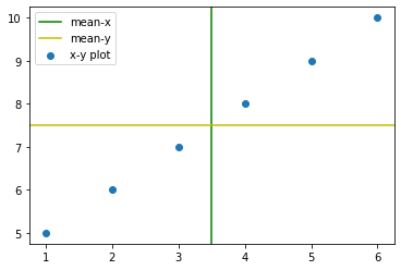
Positive Covariance#
[2]:
x = np.array([1, 2, 3, 4, 5, 6])
y = np.array([5, 6, 7, 8, 9, 10])
[3]:
plt.axvline(x.mean(),c='g',label='mean-x')
plt.axhline(y.mean(),c='y',label='mean-y')
plt.scatter(x,y,label='x-y plot')
plt.legend()
[3]:
<matplotlib.legend.Legend at 0x7f5a6a443130>
[4]:
np.sum((x- x.mean()) * (y - y.mean())) / (x.shape[0] - 1)
[4]:
3.5
[5]:
np.cov(x), np.cov(y), np.cov(x,y)
[5]:
(array(3.5),
 array(3.5),
 array([[3.5, 3.5],
        [3.5, 3.5]]))
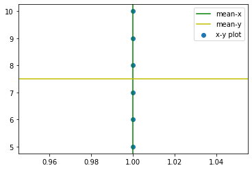
Zero Covariance#
[6]:
x = np.array([1, 1, 1, 1, 1, 1])
y = np.array([5, 6, 7, 8, 9, 10])
[7]:
plt.axvline(x.mean(),c='g',label='mean-x')
plt.axhline(y.mean(),c='y',label='mean-y')
plt.scatter(x,y,label='x-y plot')
plt.legend()
[7]:
<matplotlib.legend.Legend at 0x7f5a620c0cd0>
[8]:
np.cov(x), np.cov(y), np.cov(x,y)
[8]:
(array(0.),
 array(3.5),
 array([[0. , 0. ],
        [0. , 3.5]]))
[9]:
np.cov(x), np.cov(y), np.cov(y,x)
[9]:
(array(0.),
 array(3.5),
 array([[3.5, 0. ],
        [0. , 0. ]]))
[10]:
np.sum((x- x.mean()) * (y - y.mean())) / (x.shape[0] - 1)
[10]:
0.0
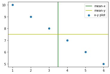
Negative Covariance#
[11]:
x = np.array([1, 2, 3, 4, 5, 6])
y = np.array([5, 6, 7, 8, 9, 10][::-1])
[12]:
plt.axvline(x.mean(),c='g',label='mean-x')
plt.axhline(y.mean(),c='y',label='mean-y')
plt.scatter(x,y,label='x-y plot')
plt.legend()
[12]:
<matplotlib.legend.Legend at 0x7f5a62033820>
[13]:
np.cov(x), np.cov(y), np.cov(x,y)
[13]:
(array(3.5),
 array(3.5),
 array([[ 3.5, -3.5],
        [-3.5,  3.5]]))
[14]:
np.sum((x- x.mean()) * (y - y.mean())) / (x.shape[0] - 1)
[14]:
-3.5
Correlation Coefficient#
How strong is the relationship between two variables.
1 indicates a strong positive relationship.
-1 indicates a strong negative relationship.
A result of zero indicates no relationship at all.
Not sensitive to the scale of data.
May not be useful if the variables don’t have linear relationship somehow.
Pearson Correlation#
\(\rho_{X,Y}=\frac{cov(X,Y)}{\sigma_X\sigma_Y}\)
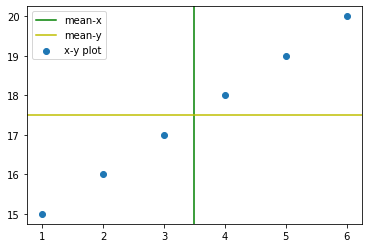
Positive Correlation#
[15]:
from scipy.stats import pearsonr
[16]:
x = np.array([1, 2, 3, 4, 5, 6])
y = np.array([15, 16, 17, 18, 19, 20])
[17]:
plt.axvline(x.mean(),c='g',label='mean-x')
plt.axhline(y.mean(),c='y',label='mean-y')
plt.scatter(x,y,label='x-y plot')
plt.legend()
[17]:
<matplotlib.legend.Legend at 0x7f5a4efaa2e0>
[18]:
cov_mat = np.cov(x,y)

print(cov_mat)
[[3.5 3.5]
 [3.5 3.5]]
[19]:
cov_mat[1][0] / np.sqrt(cov_mat[0][0] * cov_mat[1][1])
[19]:
1.0
[20]:
np.corrcoef(x,y)
[20]:
array([[1., 1.],
       [1., 1.]])
[21]:
pearsonr(x,y)
[21]:
(0.9999999999999999, 1.8488927466117464e-32)
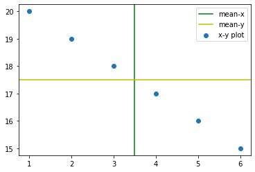
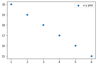
Negative Correlation#
[22]:
x = np.array([1, 2, 3, 4, 5, 6])
y = np.array([15, 16, 17, 18, 19, 20][::-1])
[23]:
plt.axvline(x.mean(),c='g',label='mean-x')
plt.axhline(y.mean(),c='y',label='mean-y')
plt.scatter(x,y,label='x-y plot')
plt.legend()
[23]:
<matplotlib.legend.Legend at 0x7f5a4ef1ca90>
[24]:
cov_mat = np.cov(x,y)

print(cov_mat)
[[ 3.5 -3.5]
 [-3.5  3.5]]
[25]:
cov_mat[1][0] / np.sqrt(cov_mat[0][0] * cov_mat[1][1])
[25]:
-1.0
[26]:
np.corrcoef(x,y)
[26]:
array([[ 1., -1.],
       [-1.,  1.]])
[27]:
np.corrcoef(x,y)[0][1]
[27]:
-1.0
[28]:
pearsonr(x,y)
[28]:
(-0.9999999999999999, 1.8488927466117464e-32)
Spearman’s Rank Correlation#
\(\rho = 1 - \frac{6 \sum {d}^2}{n(n^2 - 1)}\)
ranks#
x |
ranks |
|---|---|
1 |
1 |
2 |
2 |
3 |
3 |
4 |
4 |
x |
ranks |
|---|---|
44 |
4 |
2 |
1 |
33 |
3 |
11 |
2 |
[29]:
x = np.array([6, 4, 3, 5, 2, 1])
y = np.array([15, 16, 17, 18, 19, 20])
[30]:
def get_rank(x):
    temp = x.argsort()
    rank = np.empty_like(temp)
    rank[temp] = np.arange(len(x))
    return rank + 1
[31]:
x_rank = get_rank(x)
y_rank = get_rank(y)

print(x,x_rank)
print(y,y_rank)
[6 4 3 5 2 1] [6 4 3 5 2 1]
[15 16 17 18 19 20] [1 2 3 4 5 6]
[32]:
n = x.shape[0]
1 - ((6 * np.square(x_rank - y_rank).sum()) / (n * (n**2 - 1)))
[32]:
-0.8285714285714285
[33]:
from scipy.stats import spearmanr
[34]:
spearmanr(x,y)
[34]:
SpearmanrResult(correlation=-0.8285714285714287, pvalue=0.04156268221574334)
[35]:
plt.scatter(x,y,label='x-y plot')
plt.legend()
[35]:
<matplotlib.legend.Legend at 0x7f5a4eef8c40>
[36]:
x = np.array([1, 2, 3, 4, 5, 6])
y = np.array([15, 16, 17, 18, 19, 20])

spearmanr(x,y)
[36]:
SpearmanrResult(correlation=1.0, pvalue=0.0)
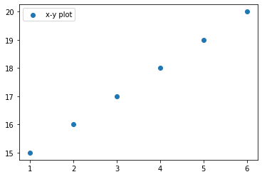
Kendall Rank Correlation (\(\tau\))#
[37]:
from scipy.stats import kendalltau
[38]:
x = np.array([1, 2, 3, 4, 5, 6])
y = np.array([15, 16, 17, 18, 19, 20])

print(kendalltau(x,y))

plt.scatter(x,y,label='x-y plot')
plt.legend()
KendalltauResult(correlation=0.9999999999999999, pvalue=0.002777777777777778)
[38]:
<matplotlib.legend.Legend at 0x7f5a4ee8f850>
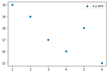
[39]:
x = np.array([1, 2, 3, 4, 5, 6])
y = np.array([15, 16, 17, 18, 19, 20][::-1])


print(kendalltau(x,y))

plt.scatter(x,y,label='x-y plot')
plt.legend()
KendalltauResult(correlation=-0.9999999999999999, pvalue=0.002777777777777778)
[39]:
<matplotlib.legend.Legend at 0x7f5a4edc1ca0>
R-Squared score / Coefficient of determination#
\(R^2 = 1 - \frac{RSS}{TSS}\)
RSS = Residual Sum of Squares = \(\sum_{i=0}^{N}{(y_i - f(x_i))^2}\)
TSS = Total Sum of Squares = \(\sum_{i=0}^{N}{(y_i - \bar{y})^2}\)
for best file of regression line will have highest r2 score.
[40]:
y = np.array([1, 2, 4, 6, 7, 9, 12, 8])
f_x = np.array([0.8, 2.2, 4, 5.9, 6.3, 9.1, 11.5, 8.5])

plt.scatter(y, f_x)
[40]:
<matplotlib.collections.PathCollection at 0x7f5a4ed3ed00>
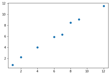
[41]:
RSS = np.square(y - f_x).sum()
TSS = np.square(y - y.mean()).sum()

print(1 - (RSS / TSS))
0.9885111989459816
[42]:
from sklearn.metrics import r2_score

r2_score(y, f_x)
[42]:
0.9885111989459816
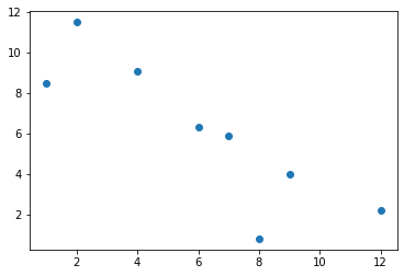
[43]:
y = np.array([1, 2, 4, 6, 7, 9, 12, 8])
f_x = np.array([0.8, 2.2, 4, 5.9, 6.3, 9.1, 11.5, 8.5][::-1])

print(r2_score(y, f_x))

plt.scatter(y,f_x)
-2.654176548089592
[43]:
<matplotlib.collections.PathCollection at 0x7f5a4e8cd250>
[44]:
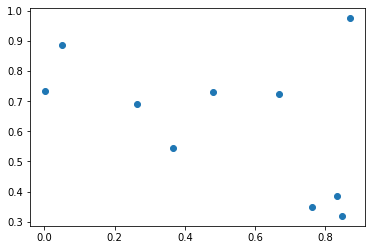
y = np.random.rand(10)
f_x = np.random.rand(10)

print(r2_score(y, f_x))

plt.scatter(y,f_x)
-1.2000772894487417
[44]:
<matplotlib.collections.PathCollection at 0x7f5a4e8a2820>