Understanding SVD#
SVD is a matrix factorization method.
basically it rotates, streches and rotates the data for various methods.(we’ll see it later)
\(X = U \Sigma V^T\)
Full SVD#
\(X_{m \times n} = U_{m \times m} \Sigma_{m \times n} V^T_{n \times n}\)
\begin{align} \begin{bmatrix} | && | && && | \\ x_1 && x_2 && ... && x_n\\ | && | && && | \\ \end{bmatrix}_{m \times n} = \begin{bmatrix} | && | && && | \\ u_1 && u_2 && .. && u_m\\ | && | && && | \\ \end{bmatrix}_{m \times m} \begin{bmatrix} \sigma_1 && 0 && 0 && 0 \\ 0 && \sigma_2 && 0 && 0 \\ && ... \\ 0 && 0 && ... && \sigma_n \\ 0 && 0 && ... && 0\\ 0 && 0 && ... && 0\\ \end{bmatrix}_{m \times n} \begin{bmatrix} -- && v_1^T && -- \\ -- && v_2^T && -- \\ && ... \\ -- && v_n^T && -- \\ \end{bmatrix}_{n \times n} \end{align}
Economy SVD#
\(X_{m \times n} = U_{m \times n} \Sigma_{n \times n} V^T_{n \times n}\)
\begin{align} \begin{bmatrix} | && | && && | \\ x_1 && x_2 && ... && x_n\\ | && | && && | \\ \end{bmatrix}_{m \times n} = \begin{bmatrix} | && | && && | \\ u_1 && u_2 && .. && u_n\\ | && | && && | \\ \end{bmatrix}_{m \times n} \begin{bmatrix} \sigma_1 && 0 && 0 && 0 \\ 0 && \sigma_2 && 0 && 0 \\ && ... \\ 0 && 0 && ... && \sigma_n \end{bmatrix}_{n \times n} \begin{bmatrix} -- && v_1^T && -- \\ -- && v_2^T && -- \\ && ... \\ -- && v_n^T && -- \\ \end{bmatrix}_{n \times n} \end{align}
\(X = \sigma_1 u_1 v_1^T + \sigma_1 u_1 v_1^T + ... + \sigma_n u_n v_n^T + 0 = \hat{U} \hat{\Sigma} \hat{V}^T\) [Till m ranks] [So actually here you just need to take m columns from U matrix because rest of them will automatically be multiplied with 0 from \(\Sigma\). It is called an economy SVD]
Properties#
\(U^T U = U U^T = I_{m \times m}\)
\(V^T V = V V^T = I_{n \times n}\) (i.e. U and V are
orthogonal, unitary matrices)\(\Sigma\) is heirarchically ordered ranks \(\sigma_1 \geq \sigma_2 \geq ... \geq \sigma_n \geq 0\) . Ordered by importance.
the columns of U are the Left singular vectors.
\(\Sigma\) (the same dimensions as A) has singular values and is
diagonal.and \(V^T\) has rows that are the Right singular vectors. The SVD represents an expansion of the original data in a coordinate system where the covariance matrix is diagonal.
_____________________    __________ ______________________
|                   |    |        ||                     |
|                   |    |        ||          V^T        |
|                   |    |        ||_____________________|
|                   |    |        | \
|         X         |  = |   U    |  \
|                   |    |        |   \ Sigma
|                   |    |        |    \
|                   |    |        |     \
|___________________|    |________|      \
Explore with numpy#
[1]:
import numpy as np
[2]:
x = np.array([
    [1, 2, 6, 8],
    [3, 4, 7, 9],
    [10, 11, 12, 13],
    [14, 15, 16, 17],
    [18, 19, 20, 21]
])
Full SVD#
[3]:
u, s, vT = np.linalg.svd(x,full_matrices=True)
[4]:
x, x.shape
[4]:
(array([[ 1,  2,  6,  8],
        [ 3,  4,  7,  9],
        [10, 11, 12, 13],
        [14, 15, 16, 17],
        [18, 19, 20, 21]]),
 (5, 4))
[5]:
m,n = x.shape
[6]:
u, u.shape # m x m
[6]:
(array([[-1.58141816e-01, -7.70036344e-01,  4.98241737e-01,
          3.65773654e-01, -5.42474680e-16],
        [-2.08984500e-01, -5.73839110e-01, -5.06126108e-01,
         -6.08991394e-01,  9.00305729e-16],
        [-4.05604099e-01,  5.92809235e-03, -5.58280362e-01,
          5.97583921e-01,  4.08248290e-01],
        [-5.45360165e-01,  1.27039223e-01, -6.73767867e-02,
          1.23438357e-01, -8.16496581e-01],
        [-6.85116231e-01,  2.48150354e-01,  4.23526789e-01,
         -3.50707206e-01,  4.08248290e-01]]),
 (5, 5))
[7]:
s, s.shape # n x 1
[7]:
(array([56.97171686, 6.33713594, 0.22186625, 0.12231847]), (4,))
[8]:
np.diag(s), np.diag(s).shape # n x n , rest of the rows till m are 0
[8]:
(array([[56.97171686,  0.        ,  0.        ,  0.        ],
        [ 0.        ,  6.33713594,  0.        ,  0.        ],
        [ 0.        ,  0.        ,  0.22186625,  0.        ],
        [ 0.        ,  0.        ,  0.        ,  0.12231847]]),
 (4, 4))
[9]:
vT, vT.shape # n x n
[9]:
(array([[-0.43544889, -0.47061031, -0.52143556, -0.56304099],
        [ 0.60168865,  0.44976548, -0.2477965 , -0.6117832 ],
        [ 0.34825926, -0.59832332,  0.62970599, -0.35241319],
        [-0.5719008 ,  0.46716822,  0.51978094, -0.42954755]]),
 (4, 4))
Assemble#
only select m columns from u. reason is explained above.
[10]:
u[:,:n] @ np.diag(s) @ vT
[10]:
array([[ 1.,  2.,  6.,  8.],
       [ 3.,  4.,  7.,  9.],
       [10., 11., 12., 13.],
       [14., 15., 16., 17.],
       [18., 19., 20., 21.]])
Economy SVD#
[11]:
u, s, vT = np.linalg.svd(x,full_matrices=False)
[12]:
x, x.shape
[12]:
(array([[ 1,  2,  6,  8],
        [ 3,  4,  7,  9],
        [10, 11, 12, 13],
        [14, 15, 16, 17],
        [18, 19, 20, 21]]),
 (5, 4))
[13]:
m,n = x.shape
[14]:
u, u.shape # m x n , rest are not required as per economy conditions
[14]:
(array([[-0.15814182, -0.77003634,  0.49824174,  0.36577365],
        [-0.2089845 , -0.57383911, -0.50612611, -0.60899139],
        [-0.4056041 ,  0.00592809, -0.55828036,  0.59758392],
        [-0.54536017,  0.12703922, -0.06737679,  0.12343836],
        [-0.68511623,  0.24815035,  0.42352679, -0.35070721]]),
 (5, 4))
[15]:
s, s.shape # n x 1
[15]:
(array([56.97171686, 6.33713594, 0.22186625, 0.12231847]), (4,))
[16]:
np.diag(s), np.diag(s).shape # n x n
[16]:
(array([[56.97171686,  0.        ,  0.        ,  0.        ],
        [ 0.        ,  6.33713594,  0.        ,  0.        ],
        [ 0.        ,  0.        ,  0.22186625,  0.        ],
        [ 0.        ,  0.        ,  0.        ,  0.12231847]]),
 (4, 4))
[17]:
vT, vT.shape # n x n
[17]:
(array([[-0.43544889, -0.47061031, -0.52143556, -0.56304099],
        [ 0.60168865,  0.44976548, -0.2477965 , -0.6117832 ],
        [ 0.34825926, -0.59832332,  0.62970599, -0.35241319],
        [-0.5719008 ,  0.46716822,  0.51978094, -0.42954755]]),
 (4, 4))
Assemble#
[18]:
u @ np.diag(s) @ vT
[18]:
array([[ 1.,  2.,  6.,  8.],
       [ 3.,  4.,  7.,  9.],
       [10., 11., 12., 13.],
       [14., 15., 16., 17.],
       [18., 19., 20., 21.]])
U & V orthogonality (Unitary matrices)#
In linear algebra, a complex square matrix U is unitary if its complexconjugate transpose U* is also its inverse, that is, if
U* U = U U* = I
\(U^T U = U U^T = I_{m \times m}\)
preserves angles and lengths of vectors
But this is true only when SVD is full, in economy one case doesnt work. See below.
References - https://en.wikipedia.org/wiki/Unitary_matrix
Full SVD#
[29]:
u, s, vT = np.linalg.svd(np.array([
    [1, 2, 3],
    [4, 5, 6],
    [7, 8, 9],
    [10,11,12]
]),full_matrices=True)
[30]:
u.T @ u
[30]:
array([[ 1.00000000e+00,  3.16686923e-16, -3.67988527e-16,
        -3.57395950e-17],
       [ 3.16686923e-16,  1.00000000e+00, -4.23968306e-16,
        -1.22189321e-17],
       [-3.67988527e-16, -4.23968306e-16,  1.00000000e+00,
        -5.06801841e-17],
       [-3.57395950e-17, -1.22189321e-17, -5.06801841e-17,
         1.00000000e+00]])
here matrix diagonal is 1. and all the other values are very close to 0.
[31]:
u @ u.T
[31]:
array([[ 1.00000000e+00, -1.77116797e-16,  1.93163256e-16,
         6.05222441e-16],
       [-1.77116797e-16,  1.00000000e+00,  5.65511925e-18,
         2.27943768e-16],
       [ 1.93163256e-16,  5.65511925e-18,  1.00000000e+00,
         2.02620226e-16],
       [ 6.05222441e-16,  2.27943768e-16,  2.02620226e-16,
         1.00000000e+00]])
[32]:
vT.T @ vT
[32]:
array([[ 1.00000000e+00, -1.17859403e-17, -2.28916495e-17],
       [-1.17859403e-17,  1.00000000e+00, -2.25135648e-16],
       [-2.28916495e-17, -2.25135648e-16,  1.00000000e+00]])
[33]:
vT @ vT.T
[33]:
array([[ 1.00000000e+00, -3.58997903e-17,  2.87055419e-16],
       [-3.58997903e-17,  1.00000000e+00,  1.07097661e-16],
       [ 2.87055419e-16,  1.07097661e-16,  1.00000000e+00]])
Economy SVD#
[34]:
u, s, vT = np.linalg.svd(np.array([
    [1, 2, 3],
    [4, 5, 6],
    [7, 8, 9],
    [10,11,12]
]),full_matrices=False)
[35]:
u.T @ u
[35]:
array([[ 1.00000000e+00,  3.16686923e-16, -3.67988527e-16],
       [ 3.16686923e-16,  1.00000000e+00, -4.23968306e-16],
       [-3.67988527e-16, -4.23968306e-16,  1.00000000e+00]])
here matrix diagonal is 1. and all the other values are very close to 0.
[36]:
u @ u.T
[36]:
array([[ 0.99926266,  0.01205509, -0.02189816,  0.01058041],
       [ 0.01205509,  0.80290688,  0.35802095, -0.17298293],
       [-0.02189816,  0.35802095,  0.34965257,  0.31422463],
       [ 0.01058041, -0.17298293,  0.31422463,  0.84817789]])
But here $U U^T$ is not Identity because in Economy SVD U matrix is not a square matrix
[37]:
vT.T @ vT
[37]:
array([[ 1.00000000e+00, -1.17859403e-17, -2.28916495e-17],
       [-1.17859403e-17,  1.00000000e+00, -2.25135648e-16],
       [-2.28916495e-17, -2.25135648e-16,  1.00000000e+00]])
[38]:
vT @ vT.T
[38]:
array([[ 1.00000000e+00, -3.58997903e-17,  2.87055419e-16],
       [-3.58997903e-17,  1.00000000e+00,  1.07097661e-16],
       [ 2.87055419e-16,  1.07097661e-16,  1.00000000e+00]])
Eckart-Young Theorem (Low rank approximation)#
Best approximation of X = \(\tilde{X}\) (X tilde)
\({{argmin}\atop{{\tilde{X} such.that. rank(\tilde{X}) = r}}} {|| X - \tilde{X} ||}_F = \tilde{U}\tilde{\Sigma}\tilde{V}^T\)
F = The Frobenius norm, sometimes also called the Euclidean norm (a term unfortunately also used for the vector -norm), is matrix norm of an matrix defined as the square root of the sum of the absolute squares of its elements.
rank r means selecting only - r columns of u - r rows of \(v^T\) - and \(\sigma\) only till r
\(\tilde{U}^T\tilde{U} = I_{r \times r}\) it is still an (r x r) identity matrix
\(\tilde{U}^T\tilde{U} \ne I_{m \times m}\) but not (m x m)
Below we are calculating approximations with rank r and Frobenius norm(Euclidean distances of the vectors, or as I understood rmse)
[24]:
x
[24]:
array([[ 1,  2,  6,  8],
       [ 3,  4,  7,  9],
       [10, 11, 12, 13],
       [14, 15, 16, 17],
       [18, 19, 20, 21]])
[25]:
u, s, vT = np.linalg.svd(x,full_matrices=False)
[26]:
r = 1

x_tilde = u[:,:r] @ np.diag(s)[:r,:r] @ vT[:r]

x_tilde , np.sqrt(np.square(x - x_tilde).sum())
[26]:
(array([[ 3.923225  ,  4.24001577,  4.69793141,  5.0727802 ],
        [ 5.18454406,  5.60318323,  6.20831901,  6.70368189],
        [10.06233633, 10.87484522, 12.04931296, 13.0107298 ],
        [13.52944265, 14.62191184, 16.20105742, 17.49374269],
        [16.99654897, 18.36897847, 20.35280189, 21.97675558]]),
 6.342198225330375)
[27]:
r = 2

x_tilde = u[:,:r] @ np.diag(s)[:r,:r] @ vT[:r]

x_tilde , np.sqrt(np.square(x - x_tilde).sum())
[27]:
(array([[ 0.98708971,  2.04523896,  5.90713494,  8.05817515],
        [ 2.99650543,  3.96761267,  7.10943008,  8.92842933],
        [10.08494004, 10.89174162, 12.04000396, 12.98774686],
        [14.01384101, 14.98400221, 16.00156518, 17.00121755],
        [17.94274198, 19.0762628 , 19.9631264 , 21.01468825]]),
 0.253350433705557)
[28]:
r = 3

x_tilde = u[:,:r] @ np.diag(s)[:r,:r] @ vT[:r]

x_tilde , np.sqrt(np.square(x - x_tilde).sum())
[28]:
(array([[ 1.02558734,  1.97909849,  5.97674455,  8.01921833],
        [ 2.9573986 ,  4.03479978,  7.03871895,  8.96800262],
        [10.0418034 , 10.96585208, 11.96200633, 13.03139801],
        [14.00863501, 14.99294632, 15.99215194, 17.00648565],
        [17.97546662, 19.02004057, 20.02229755, 20.98157328]]),
 0.12231846893897867)
[29]:
r = 4

x_tilde = u[:,:r] @ np.diag(s)[:r,:r] @ vT[:r]

x_tilde , np.sqrt(np.square(x - x_tilde).sum())
[29]:
(array([[ 1.,  2.,  6.,  8.],
        [ 3.,  4.,  7.,  9.],
        [10., 11., 12., 13.],
        [14., 15., 16., 17.],
        [18., 19., 20., 21.]]),
 2.3593480078153382e-14)
SVD and Correlations#
This is an interpretation of SVD. Not a very good computation method
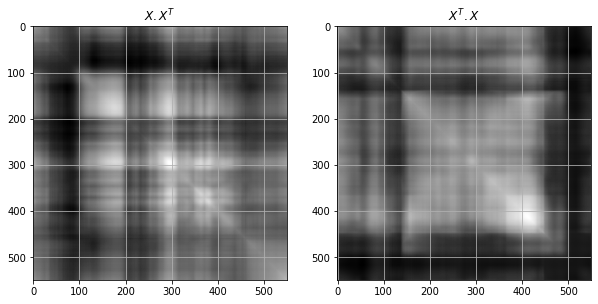
\begin{align} X^TX=\begin{bmatrix} -- && x_1^T && --\\ -- && x_2^T && --\\ && .\\ && .\\ -- && x_n^T && --\\ \end{bmatrix}_{n \times m} \begin{bmatrix} | && | && && |\\ x_1 && x_2 && ... && x_n\\ | && | && && |\\ \end{bmatrix}_{m \times n}= \begin{bmatrix} x_1^T x_1 && x_1^T x_2 && ... && x_1^T x_n\\ x_2^T x_1 && x_2^T x_2 && ... && x_2^T x_n\\ . && . && ... && .\\ x_n^T x_1 && x_n^T x_2 && ... && x_n^T x_n\\ \end{bmatrix}_{n \times n} \end{align}
here we are calculating product of columns actually. observe the first row of the left matrix is actually the column of the original matrix and by matrix multiplication it is getting multiplied to the first column of the right matrix
if \(X = U \Sigma V^T\)
then \(X^T = V \Sigma U^T\)
\(X^T X = V \Sigma U^T U \Sigma V^T = V \Sigma^2 V^T\)
multiplying V both sides
\(X^T X V = V \Sigma^2\)
\begin{align} XX^T=\begin{bmatrix} | && | && && |\\ x_1 && x_2 && ... && x_n\\ | && | && && |\\ \end{bmatrix}_{m \times n} \begin{bmatrix} -- && x_1^T && --\\ -- && x_2^T && --\\ && .\\ && .\\ -- && x_n^T && --\\ \end{bmatrix}_{n \times m}= \begin{bmatrix} x_1x_1^T && x_2 x_1^T && ... && x_1^T x_m\\ x_2^T x_1 && x_2 x_2^T && ... && x_2^T x_m\\ . && . && ... && .\\ x_m^T x_1 && x_2 x_m^T && ... && x_m^T x_m\\ \end{bmatrix}_{m \times m} \end{align}
here we are calculating product of rows
\(X X^T = U \Sigma V^T V \Sigma U^T = U \Sigma^2 U^T\)
multiplying U both sides \(X^T X U = U \Sigma^2\)
Now using this explanation to calculate SVD
Method of Snapshots (SVD using eigen values and vectors)#
for U
calculate X * \(X^T\)
calculate eigen values and vectors
U = eigen vectors of X * \(X^T\)
for V
calculate \(X^T\) * X
calculate eigen values and vectors
V = eigen vectors of \(X^T\) * X
[30]:
x_xT = x @ x.T
U_values, U = np.linalg.eig(x_xT)
eigen vector for U
[31]:
print(U)
[[ 1.58141816e-01 -7.70036344e-01  4.98241737e-01  3.65773654e-01
   1.66017468e-13]
 [ 2.08984500e-01 -5.73839110e-01 -5.06126108e-01 -6.08991394e-01
  -2.51244615e-13]
 [ 4.05604099e-01  5.92809235e-03 -5.58280362e-01  5.97583921e-01
   4.08248290e-01]
 [ 5.45360165e-01  1.27039223e-01 -6.73767867e-02  1.23438357e-01
  -8.16496581e-01]
 [ 6.85116231e-01  2.48150354e-01  4.23526789e-01 -3.50707206e-01
   4.08248290e-01]]
eigen value of U
[32]:
print(U_values)
[3.24577652e+03 4.01592919e+01 4.92246344e-02 1.49618078e-02
 5.41176252e-16]
[33]:
xT_x = x.T @ x

V_values, V = np.linalg.eig(xT_x)
eigen vector of V
[34]:
print(V.T)
[[ 0.43544889  0.47061031  0.52143556  0.56304099]
 [-0.60168865 -0.44976548  0.2477965   0.6117832 ]
 [ 0.5719008  -0.46716822 -0.51978094  0.42954755]
 [-0.34825926  0.59832332 -0.62970599  0.35241319]]
eigen value of V
[35]:
print(V_values)
[3.24577652e+03 4.01592919e+01 1.49618078e-02 4.92246344e-02]
singular value : square root of U values in descending order
[36]:
singular_val = np.sqrt(U_values.real[:-1])
np.sort(singular_val)[::-1]
[36]:
array([56.97171686, 6.33713594, 0.22186625, 0.12231847])
Vector outer product#
\(a=\begin{bmatrix} a_0 && a_1 && ... && a_m \end{bmatrix}\)
\(b=\begin{bmatrix} b_0 && b_1 && ... && b_n \end{bmatrix}\)
Vector outer product = \(\begin{bmatrix} a_0b_0 && a_0b_1 && ... && a_0b_n\\ a_1b_0 && a_1b_1 && ... && a_1b_n\\ && ... && ... &&\\ a_mb_0 && a_mb_1 && ... && a_mb_n\\ \end{bmatrix}\)
Example - \(\begin{bmatrix} 3 && 4\\ \end{bmatrix} \begin{bmatrix} 5 && 6\\ \end{bmatrix}= \begin{bmatrix} 3 \\ 4 \end{bmatrix} \begin{bmatrix} 5 && 6 \end{bmatrix}= \begin{bmatrix} 3 \times 5 && 3 \times 6 \\ 4 \times 5 && 4 \times 6 \end{bmatrix}= \begin{bmatrix} 15 && 18 \\ 20 && 24 \end{bmatrix}\)
[37]:
np.outer(np.array([3,4]),np.array([5,6]))
[37]:
array([[15, 18],
       [20, 24]])
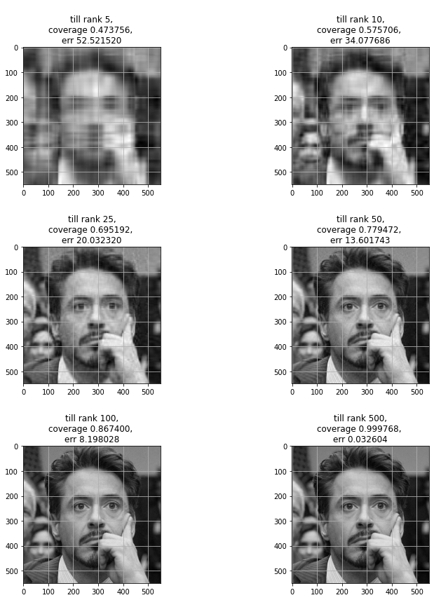
SVD and Image Compression#
In simple words choosing lowest rank index(ranks are in descending order) required to generate a close approximation original matrix.
[38]:
import matplotlib.pyplot as plt

plt.rcParams.update({
    "axes.grid": True
})

%matplotlib inline
[39]:
img = plt.imread('./images/rdj.jpg') / 255
[40]:
gray_img = np.mean(img,axis=2) #2 because I know this is a 3D matrix. I can give -1 to take the maximum dimension
[41]:
plt.imshow(gray_img,cmap='gray')
[41]:
<matplotlib.image.AxesImage at 0x7f13e62af9a0>

[42]:
gray_img.shape
[42]:
(550, 550)
[43]:
%matplotlib inline

fig = plt.figure(figsize=(10,5))
ax = fig.subplots(1,2)

ax[0].set_title(f"$X . X^T$")
ax[0].imshow(gray_img @ gray_img.T, cmap='gray')

ax[1].set_title(f"$X^T . X$")
ax[1].imshow(gray_img.T @ gray_img, cmap='gray')
[43]:
<matplotlib.image.AxesImage at 0x7f13e479f640>
[44]:
u,s,vT = np.linalg.svd(gray_img,full_matrices=True)

ranks = [5,10,25,50,100,500]
Log and Cumulative plots#
log plot will show to keep the first few ranks and throw rest of them as thier rank/ importance is not that much.
cumulative plots purpose is to see that at what rank what percentage of the original matrix values(energy) is getting covered. on x axis = ranks on y axis = \(\frac{\sum_{i=0}^{r}{\sigma_i}}{\sum_{i=0}^{m}{\sigma_i}}\)
to pick up a rank where we can get maximum energy possible
[45]:
%matplotlib inline

fig,ax = plt.subplots(1,2,figsize=(15,5))

ax[0].set(xlabel='ranks',ylabel='log($\sigma$)')
for rank in ranks:
    ax[0].axvline(rank)
ax[0].plot(np.log(s),'k.-')

ax[1].set(xlabel='ranks',ylabel='Cumulative energy ($\sigma$)')
for rank in ranks:
    ax[1].axvline(rank)
ax[1].plot(np.cumsum(s)/np.sum(s),'k.-')
[45]:
[<matplotlib.lines.Line2D at 0x7f13e4614580>]
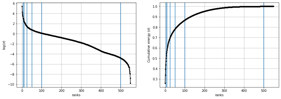
we can see around at rank 100, approx 90% original matrix is recovered.
[46]:
def calc_c_mat(u,s,vT,r):
    """Compressed matrix calculation.
    """
    return u[:,:r] @ np.diag(s)[:r,:r] @ vT[:r]

def calc_cum_enery_percentage(s,r):
    return np.sum(s[:r])/np.sum(s)

def rmse(x,x_bar):
    return np.sqrt(np.square(x - x_bar).sum())
[47]:
%matplotlib inline

fig,ax = plt.subplots(3,2,figsize=(12,12))

r = ranks[0]
c_img = calc_c_mat(u,s,vT,r)
err = rmse(gray_img,c_img)
cov = calc_cum_enery_percentage(s,r)
ax[0][0].set_title(f"""
till rank {r},
coverage {cov:2f},
err {err:2f}""")
ax[0][0].imshow(c_img,cmap='gray')

r = ranks[1]
c_img = calc_c_mat(u,s,vT,r)
err = rmse(gray_img,c_img)
cov = calc_cum_enery_percentage(s,r)
ax[0][1].set_title(f"""
till rank {r},
coverage {cov:2f},
err {err:2f}""")
ax[0][1].imshow(c_img,cmap='gray')

r = ranks[2]
c_img = calc_c_mat(u,s,vT,r)
err = rmse(gray_img,c_img)
cov = calc_cum_enery_percentage(s,r)
ax[1][0].set_title(f"""
till rank {r},
coverage {cov:2f},
err {err:2f}""")
ax[1][0].imshow(c_img,cmap='gray')


r = ranks[3]
c_img = calc_c_mat(u,s,vT,r)
err = rmse(gray_img,c_img)
cov = calc_cum_enery_percentage(s,r)
ax[1][1].set_title(f"""
till rank {r},
coverage {cov:2f},
err {err:2f}""")
ax[1,1].imshow(c_img,cmap='gray')

r = ranks[4]
c_img = calc_c_mat(u,s,vT,r)
err = rmse(gray_img,c_img)
cov = calc_cum_enery_percentage(s,r)
ax[2][0].set_title(f"""
till rank {r},
coverage {cov:2f},
err {err:2f}""")
ax[2][0].imshow(c_img,cmap='gray')

r = ranks[5]
c_img = calc_c_mat(u,s,vT,r)
err = rmse(gray_img,c_img)
cov = calc_cum_enery_percentage(s,r)
ax[2][1].set_title(f"""
till rank {r},
coverage {cov:2f},
err {err:2f}""")
ax[2][1].imshow(c_img,cmap='gray')

plt.tight_layout()
Rotation matrix#
In linear algebra, a rotation matrix is a transformation matrix that is used to perform a rotation in Euclidean space. For example, using the convention below, the matrix for
2D Rotation
\(R(\theta) = \begin{bmatrix} cos\theta && -sin\theta\\ sin\theta && cos\theta \end{bmatrix}\)
3D Rotation
\(R_x(\theta) = \begin{bmatrix} 1 && 0 && 0\\ 0 && cos\theta && -sin\theta\\ 0 && sin\theta && cos\theta \end{bmatrix}\)
\(R_y(\theta) = \begin{bmatrix} cos\theta && 0 && sin\theta\\ 0 && 1 && 0\\ -sin\theta && 0 && cos\theta \end{bmatrix}\)
\(R_z(\theta) = \begin{bmatrix} cos\theta && -sin\theta && 0\\ sin\theta && cos\theta && 0\\ 0 && 0 && 1\\ \end{bmatrix}\)
\(R(\theta) = R_x(\theta) R_y(\theta) R_z(\theta)\)
References- https://en.wikipedia.org/wiki/Rotation_matrix
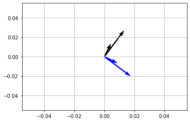
Rotating vectors \(90^\circ\) or \(\pi/2\)#
[48]:
theta = np.pi/2

R = np.array([
    [ np.cos(theta), -np.sin(theta) ],
    [ np.sin(theta), np.cos(theta) ]
])

vec = np.array([
    [1, 2],
    [3, 4]
])


vecR = vec @ R #multiply rotation matrix with vector matrix

x,y = vec[...,[0]],vec[...,[1]]
Rx, Ry = vecR[...,[0]],vecR[...,[1]]
fig,ax = plt.subplots(1,1)

ax.quiver(*np.zeros_like(vec.T),x,y,scale=25)
ax.quiver(*np.zeros_like(vecR.T),Rx,Ry,scale=25,color='blue')

plt.show()
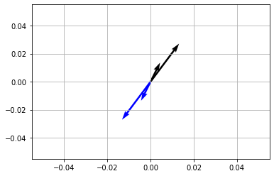
Rotating vectors \(180^\circ\) or \(\pi\)#
[49]:
theta = np.pi

R = np.array([
    [ np.cos(theta), -np.sin(theta) ],
    [ np.sin(theta), np.cos(theta) ]
])

vec = np.array([
    [1, 2],
    [3, 4]
])


vecR = vec @ R

x,y = vec[...,[0]],vec[...,[1]]
Rx, Ry = vecR[...,[0]],vecR[...,[1]]
fig,ax = plt.subplots(1,1)

ax.quiver(*np.zeros_like(vec.T),x,y,scale=25)
ax.quiver(*np.zeros_like(vecR.T),Rx,Ry,scale=25,color='blue')

plt.show()
Unitary transformation#
rotate vectors , dont change angles between them
\(< x, y > = < Ux, Uy > \forall{x,y}\in\mathbf{R}\)
<,> = inner product
Ux = unitary transformed x
Uy = unitary transformed y
if X \(\in \mathbf{C}\) complex then X* is complex conjugate transpose.
|461702cc93434f149d67129b7a2070e3|
[62]:
from mpl_toolkits import mplot3d
[198]:
import matplotlib.pyplot as plt
%matplotlib inline
[199]:
# theta = [np.pi/15, -np.pi/9, -np.pi/20]

theta = [np.pi/4,np.pi/4,np.pi/4]


# rotation on x
Rx = np.array([
    [1, 0, 0],
    [0, np.cos(theta[0]), -np.sin(theta[0])],
    [0, np.sin(theta[0]), np.cos(theta[0])]
])

# rotation on y
Ry = np.array([
    [np.cos(theta[1]), 0, np.sin(theta[1])],
    [0, 1, 0],
    [-np.sin(theta[1]), 0, np.cos(theta[1])]
])

# rotation on z
Rz = np.array([
    [np.cos(theta[2]), -np.sin(theta[2]), 0],
    [np.sin(theta[2]), np.cos(theta[2]), 0],
    [0, 0, 1]
])

# stretch
Sigma = np.diag([5, 3, 1])

X = Rz @ Ry @ Rx @ Sigma

U, S, VT = np.linalg.svd(X,full_matrices=False)
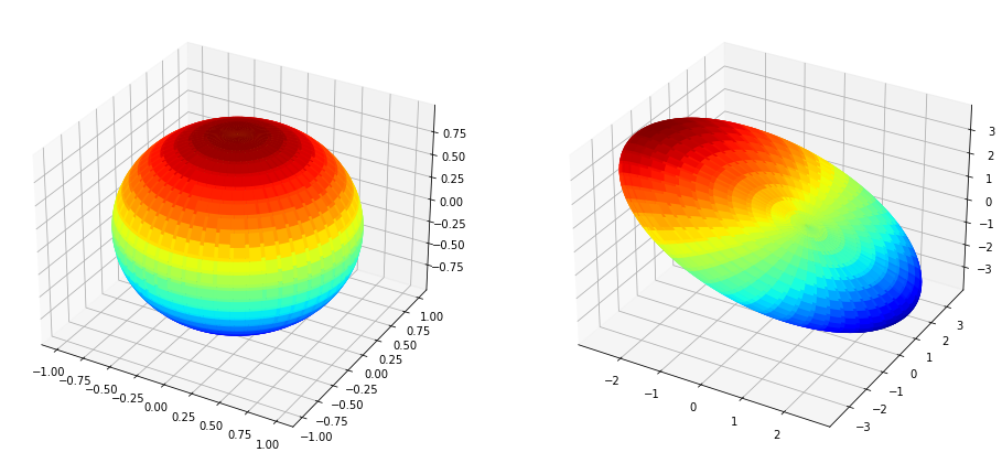
Multiplying by X#
[200]:
plt.rcParams["figure.figsize"] = (16, 8)

u = np.linspace(-np.pi,np.pi, 100)
v = np.linspace(-np.pi,np.pi, 100)

x = np.outer(np.cos(u),np.cos(v))
y = np.outer(np.sin(u),np.cos(v))
z = np.outer(np.ones_like(u),np.sin(v))

fig = plt.figure()
ax1 = fig.add_subplot(121,projection='3d')

ax1.plot_surface(x, y, z, cmap='jet')


xR = np.zeros_like(x)
yR = np.zeros_like(y)
zR = np.zeros_like(z)

rows,columns = x.shape

for row in range(rows):
    for col in range(columns):
        vec = [ x[row,col], y[row,col], z[row,col] ]

        vecR = X @ vec
        xR[row, col] = vecR[0]
        yR[row, col] = vecR[1]
        zR[row, col] = vecR[2]

ax2 = fig.add_subplot(122,projection='3d')

ax2.plot_surface(xR, yR, zR, cmap='jet')

plt.show()
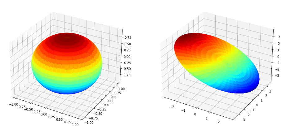
Multiplying by \(U\Sigma\)#
[204]:
plt.rcParams["figure.figsize"] = (16, 8)

u = np.linspace(-np.pi,np.pi, 100)
v = np.linspace(-np.pi,np.pi, 100)

x = np.outer(np.cos(u),np.cos(v))
y = np.outer(np.sin(u),np.cos(v))
z = np.outer(np.ones_like(u),np.sin(v))

fig = plt.figure()
ax1 = fig.add_subplot(121,projection='3d')

ax1.plot_surface(x, y, z, cmap='jet')


xR = np.zeros_like(x)
yR = np.zeros_like(y)
zR = np.zeros_like(z)

rows,columns = x.shape

for row in range(rows):
    for col in range(columns):
        vec = [ x[row,col], y[row,col], z[row,col] ]

        vecR = U @ np.diag(S) @ vec
        xR[row, col] = vecR[0]
        yR[row, col] = vecR[1]
        zR[row, col] = vecR[2]

ax2 = fig.add_subplot(122,projection='3d')

ax2.plot_surface(xR, yR, zR, cmap='jet')

plt.show()
[ ]: