
Loss Functions#
References#
https://en.wikipedia.org/wiki/Loss_functions_for_classification
https://www.cs.cornell.edu/courses/cs4780/2018fa/lectures/lecturenote10.html
[1]:
import numpy as np
from sklearn import metrics

import matplotlib.pyplot as plt

plt.style.use("fivethirtyeight")
Loss vs Cost Function#
\begin{align} \text{Cost Function } J(h_w(X), y) = \frac{1}{N} \sum_{i=1}^{N} L(h_w(x_i), y_i) \end{align}
Classification Loss#
Hinge Loss#
\begin{align} L(h_w(x_i), y_i) = \max(1 - h_w(x_i) y_i, 0)^p \end{align}
p |
Usecase |
|---|---|
p = 1 |
SVM |
p = 2 |
Squared Loss SVM |
Generally used for Standard SVM
[23]:
def hinge_loss(y_true, y_pred, p):
    return np.power(np.max(np.c_[1 - (y_true * y_pred), np.zeros_like(y_true)], axis=1), p)
Correct classification
[29]:
hinge_loss(-1, -1, 1), hinge_loss(-1, -1, 2)
[29]:
(array([0]), array([0]))
Incorrect Classification
[31]:
hinge_loss(-1, 1, 1), hinge_loss(1, -1, 1)
[31]:
(array([2]), array([2]))
[41]:
y_true = np.array([1, -1, 1, -1, 1, -1, 1, -1, 1])
y_pred = np.array([-1, -1, 1, -1, 1, -1, -1, -1, 1])

metrics.hinge_loss(y_pred, y_true), hinge_loss(y_true, y_pred, 1).mean()
[41]:
(0.4444444444444444, 0.4444444444444444)
[42]:
metrics.hinge_loss([-1], [-1]), metrics.hinge_loss([-1], [1])
[42]:
(0.0, 2.0)
Log Loss#
\begin{align} L(h_w(x_i), y_i) = \log(1 + e^{- y_i h_w(x_i)}) \end{align}
Used for Logistic Regression
[43]:
def logistic_loss(y_true, y_pred):
    return np.log(1 + np.exp(-(y_true * y_pred)))

def log_loss(y_true, y_pred):
    return ((y_true * np.log(y_pred)) + ((1 - y_true) * np.log(1 - y_pred)))
Correct classification
[45]:
logistic_loss(-1, -1), logistic_loss(1, 1)
[45]:
(0.31326168751822286, 0.31326168751822286)
Incorrect Classification
[46]:
logistic_loss(-1, 1), logistic_loss(1, -1)
[46]:
(1.3132616875182228, 1.3132616875182228)
[55]:
y_true = np.array([1, -1, 1, -1, 1, -1, 1, -1, 1])
y_pred = np.array([-1, -1, 1, -1, 1, -1, -1, -1, 1])

logistic_loss(y_true, y_pred).mean()
[55]:
0.535483909740445
Exponential Loss#
\begin{align} L(h_w(x_i), y_i) = e^{-h_w(x_i) y_i} \end{align}
Adaboost
Very aggressive, Loss of misprediction increases exponentially
[56]:
def exp_loss(y_true, y_pred):
    return np.exp(-(y_pred * y_true))
Correct classification
[57]:
exp_loss(-1, -1), exp_loss(1, 1)
[57]:
(0.36787944117144233, 0.36787944117144233)
Incorrect Classification
[58]:
exp_loss(-1, 1), exp_loss(1, -1)
[58]:
(2.718281828459045, 2.718281828459045)
[59]:
y_true = np.array([1, -1, 1, -1, 1, -1, 1, -1, 1])
y_pred = np.array([-1, -1, 1, -1, 1, -1, -1, -1, 1])

exp_loss(y_true, y_pred).mean()
[59]:
0.8901910827909096
Zero-One Loss#
\begin{align} L(h_w(x_i), y_i) &= \delta(sign({h_w(x_i)) \ne y_i}) \\ \\ \delta &= \begin{cases} 1 & \text{if } sign(h_w(x_i)) \ne y_i \text{ i.e. missclassification}\\ \\ 0 & \text{otherwise} \end{cases} \end{align}
Actual Classification loss
[60]:
def zero_one_loss(y_true, y_pred):
    return np.int32(np.sign(y_pred) != y_true)
Correct classification
[61]:
zero_one_loss(-1, -1), zero_one_loss(1, 1)
[61]:
(0, 0)
Incorrect Classification
[62]:
zero_one_loss(-1, 1), zero_one_loss(-1, 1)
[62]:
(1, 1)
[63]:
y_true = np.array([1, -1, 1, -1, 1, -1, 1, -1, 1])
y_pred = np.array([-1, -1, 1, -1, 1, -1, -1, -1, 1])

zero_one_loss(y_true, y_pred).mean()
[63]:
0.2222222222222222
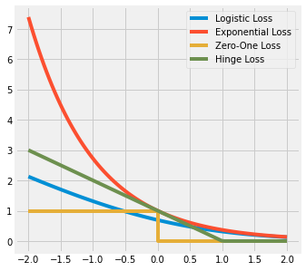
Graphical Representation#
[70]:
n_samples = 100

x = np.linspace(-2, 2, n_samples)
y = np.ones_like(x)

fig, ax = plt.subplots(1, 1, figsize=(5, 5))

ax.plot(x, logistic_loss(x, y), label='Logistic Loss')
ax.plot(x, exp_loss(x, y), label='Exponential Loss')
ax.plot(np.int32(x), zero_one_loss(y, x), label='Zero-One Loss')
ax.plot(x, hinge_loss(x, y, 1), label='Hinge Loss')

plt.legend()
plt.show()
Regression Loss#
Squared Loss#
\begin{align} L(h_w(x_i), y_i) &= (h_w(x_i) - y_i)^2 \end{align}
also known as
Ordinary Least Squareestimates mean label
Differenciable easily
affected by noisy data
[17]:
def squared_loss(y_true, y_pred):
    return np.square(y_pred - y_true)
[72]:
y_true = np.array([12, 11, 10, 12.3, 11.2, 10.3])
y_pred = np.array([11.9, 11, 9.6, 12, 11, 10.1])

squared_loss(y_true, y_pred).mean(), metrics.mean_squared_error(y_true, y_pred)
[72]:
(0.05666666666666679, 0.05666666666666679)
Absolute Loss#
\begin{align} L(h_w(x_i), y_i) &= |h_w(x_i) - y_i| \end{align}
Estimates median label
Less sensitive to noise
[73]:
def absolute_loss(y_true, y_pred):
    return np.abs(y_pred - y_true)
[74]:
y_true = np.array([12, 11, 10, 12.3, 11.2, 10.3])
y_pred = np.array([11.9, 11, 9.6, 12, 11, 10.1])

absolute_loss(y_true, y_pred).mean(), metrics.mean_absolute_error(y_true, y_pred)
[74]:
(0.20000000000000018, 0.20000000000000018)
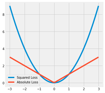
Graphical Representation#
[84]:
n_samples = 50

x = np.linspace(-3, 3, n_samples)
y = np.zeros_like(x)

fig, ax = plt.subplots(1, 1, figsize=(5, 5))

ax.plot(x, squared_loss(x, y), label='Squared Loss')
ax.plot(x, absolute_loss(x, y), label='Absolute Loss')

plt.legend()
plt.show()
[ ]: