SVD,Linear Systems and Least Square

Linear System of equations \(X\theta=Y\)

X and Y is known where \(\theta\) to be found.

In most cases X is square matrix and invertible but SVD helps us to generalize solution for non square X

Non-square matrices (m-by-n matrices for which m ≠ n) do not have an inverse. A square matrix that is not invertible is called singular or degenerate. A square matrix is singular if and only if its determinant is 0.

In linear algebra an n-by-n (square) matrix A is called invertible (some authors use nonsingular or nondegenerate)

There the term psuedo inverse comes in picture, where we use SVD to calculate the inverse of a non square matrix.

Types of Non-Square Matrix solutions

m = number of samples(number of rows)

n = number of features(number of columns)

Underdetermined (m<n)

               X                  𝜃     Y
 ______________________________   _     _
|        SHORT                 | | | = | |
|        FAT                   | | |   | |
|______________________________| | |   |_|
                                 | |
                                 | |
                                 |_|

In general \(\infty\) many solutions of \(\theta\) given Y. as there are not enough samples available of Y to determine \(\theta\). But again there are cases where solution is possible. We’ll understand more about this later.

Overdetermined (m>n)

       X          𝜃     Y
 ______________   _     _
|     TALL     | | | = | |
|    SKINNY    | | |   | |
|              | | |   | |
|              | | |   | |
|              | | |   | |
|              | |_|   | |
|              |       | |
|              |       | |
|______________|       |_|

In general 0 solution of \(\theta\) given Y. But again we can cook up matrix that generates a solution.

This is where SVD helps, It generates the best approximate psuedo inverse that gives us a result for \(\theta\) for best fit.

Minimum Norm Solution

for underdetermined cases

\({{min || \tilde{\theta} ||_2}\atop{\text{minimum norm soln}}} {s.t. X \tilde{\theta} = Y}\)

It is like cheapest way to multiply matrix X to \(\theta\)

I am not sure If I understand this

Least Squares Solution (Calculating \(\tilde{\theta}\))

for overdetermined cases

\(minimize || X \tilde{\theta} - Y ||_2\)

\(X = \hat{U} \hat{\Sigma} \hat{V}^T (\text{economy})\)

\begin{align} & X \tilde{\theta} = Y \\ & \hat{U} \hat{\Sigma} \hat{V}^T \tilde{\theta} = Y\\ & \hat{V} \hat{\Sigma}^{-1} \hat{U}^T \hat{U} \hat{\Sigma} \hat{V}^T \tilde{\theta} = \hat{V} \hat{\Sigma}^{-1} \hat{U}^T Y\\ & \tilde{\theta} = \hat{V} \hat{\Sigma}^{-1} \hat{U}^T Y \end{align}

where \begin{align} \hat{U}^T \hat{U} = I\\ \hat{\Sigma}^{-1} \hat{\Sigma} = I\\ \hat{V} \hat{V}^T = I \end{align}

Moore-Penrose Inverse

\(X^\dagger = V \Sigma^{-1} U^T\)

It is called the Moore–Penrose inverse. where \(X^\dagger\)(X-dagger) is psuedo inverse.

But what happens when we again multiply \(\tilde{\theta}\) to X ?

\begin{align} X \tilde{\theta} \\ \hat{U} \hat{\Sigma} \hat{V}^T \hat{V} \hat{\Sigma}^{-1} \hat{U}^T Y \\ \hat{U} \hat{U}^T Y \end{align}

because \begin{align} \hat{V}^T \hat{V} = I \\ \hat{\Sigma} \hat{\Sigma}^{-1} = I\\ \text{but} && \hat{U} \hat{U}^T \ne I \end{align}

because It is an economy SVD and in economy SVD U matrix is not a square matrix. For proof see SVD doc.

This is the reason why the result is not exactly Y.

projection of Y onto span(U) [Columns of U] and that means span(X) [Columns of X]

Understanding spaces

Solution of \(X \theta = Y\) exists only and only if Y is in column space of X.

where

• Column space of A [col(A)] = Column space of \(\hat{U}\) [col(\(\hat{U}\))] … range

• Kernel of \(A^T\) [ker(\(A^T\))] … orthogonal compliment to col(A) (The orthogonal complement is a subspace of vectors where all of the vectors in it are orthogonal to all of the vectors in a particular subspace. For instance, if you are given a plane in ℝ³, then the orthogonal complement of that plane is the line that is normal to the plane and that passes through (0,0,0).)

• Row space of A [row(A)] = Row space of \(V^T\) [row(\(V^T\))] = Column space of V [col(V)]

• Kernel of A [ker(A)] … null space (In mathematics, the kernel of a linear map, also known as the null space or nullspace, is the linear subspace of the domain of the map which is mapped to the zero vector.)

TODO

Calculate with Data

import numpy as np
import matplotlib.pyplot as plt
from mpl_toolkits import mplot3d

from sklearn.datasets import make_regression

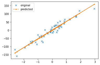
With 1 Feature

X,Y = make_regression(n_samples=50,n_features=1,noise=20)

Y = Y.reshape(-1,1)

X.shape, Y.shape

((50, 1), (50, 1))

U,S,VT = np.linalg.svd(X,full_matrices=False)

U.shape, S.shape, VT.shape

((50, 1), (1,), (1, 1))

theta_tilde = VT.T @ np.linalg.pinv(np.diag(S)) @ U.T @ Y

Y_pred = X @ theta_tilde

%matplotlib inline


plt.plot(X[...,0],Y,'x',label='original')
plt.plot(X[...,0],Y_pred,'.--',label='predicted')

plt.legend()
plt.show()

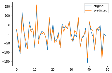
plt.plot(Y,label='original')
plt.plot(Y_pred,label='predicted')

plt.legend()
plt.show()

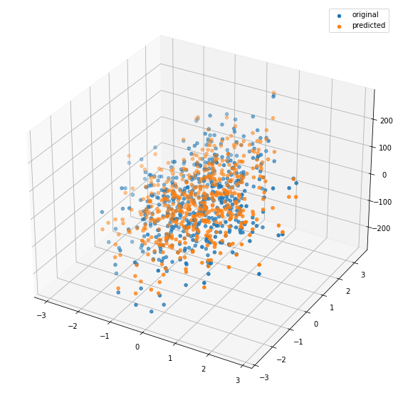
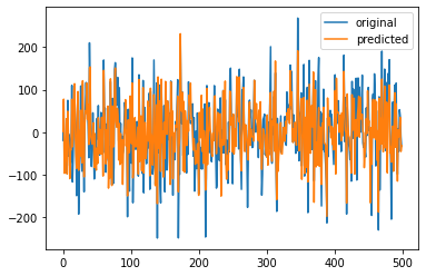
With 2 features

X,Y = make_regression(n_samples=500,n_features=2,noise=50)

Y = Y.reshape(-1,1)

X.shape, Y.shape

((500, 2), (500, 1))

U,S,VT = np.linalg.svd(X,full_matrices=False)

U.shape, S.shape, VT.shape

((500, 2), (2,), (2, 2))

theta_tilde = VT.T @ np.linalg.pinv(np.diag(S)) @ U.T @ Y

Y_pred = X @ theta_tilde

%matplotlib inline

fig = plt.figure(figsize=(10,10))
ax = plt.axes(projection='3d')

ax.scatter(X[...,0],X[...,1],Y, cmap='viridis',label='original')
ax.scatter(X[...,0],X[...,1],Y_pred, cmap='viridis',label='predicted')

plt.legend()
plt.show()

plt.plot(Y,label='original')
plt.plot(Y_pred,label='predicted')

plt.legend()
plt.show()

Another method to calcualte \(\tilde{\theta}\)

\(X \theta = Y\)

\(\tilde{\theta} = pinv(X) Y\)

theta_tilde2 = np.linalg.pinv(X) @ Y

Y_pred = X @ theta_tilde2

plt.plot(Y,label='original')
plt.plot(Y_pred,label='predicted')

plt.legend()
plt.show()

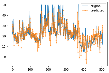
Boston housing data regression analysis

from sklearn.datasets import load_boston

dataset = load_boston()

X,Y = dataset.data,dataset.target.reshape(-1,1)

X.shape, Y.shape

((506, 13), (506, 1))

U, S, VT = np.linalg.svd(X,full_matrices=False)

theta_tilde = VT.T @ np.linalg.pinv(np.diag(S)) @ U.T @ Y

Y_pred = X @ theta_tilde

plt.plot(Y,label='original')
plt.plot(Y_pred,'.-',label='predicted',alpha=0.6)

plt.legend()
plt.show()